DLEGOS / EQUATIONS TO EXECUTABLE MODELS
Mathematical development laboratory
Derive the update. Verify the solver. Learn one closure. Inspect the budget.
Executed constructed experiments only. This is a small numerical-development companion, not a trained Caribbean weather model.
Loading archived coefficients…
1. State, geometry and units
Start with a specific physical object rather than a general list of equations. The executable system is a closed chain of twelve well-mixed thermal cells with eleven internal faces. Each cell stores a temperature T in K and a positive capacity C in J K⁻¹. Each edge has one orientation and one non-negative conductance G in W K⁻¹. There is no boundary heating, radiation, humidity, resolved wind or precipitation. The small capacities are constructed values chosen for numerical development; they do not approximate the heat capacity of a kilometre-wide atmospheric cell.
The incidence matrix B is node-by-edge, with −1 at the sender and +1 at the receiver. For a column state, ΔT=BᵀT and q=−G⊙ΔT. The node energy tendency is Bq and the node temperature tendency is C⁻¹Bq. With this convention a hotter sender produces a positive transfer towards a cooler receiver. Reversing the arbitrary edge orientation changes both the gradient and the bookkeeping signs, so the physical result is unchanged.
difference = T @ B                 # batch × edge
edge_power = -difference * G        # W
node_tendency = (edge_power @ B.T) / C  # K/s
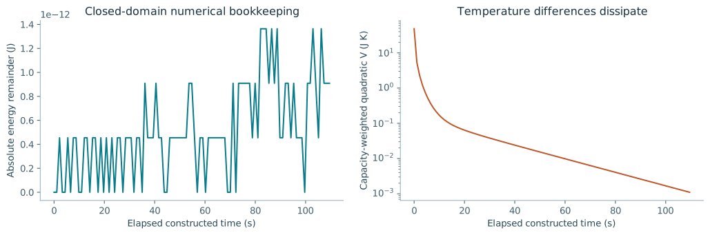
Before learning, verify B’s shape, the identity 1ᵀB=0 and a zero tendency for a constant-temperature field. Then verify pairwise exchange with unequal capacities. The capacity-weighted domain temperature, not the arithmetic mean, determines the equilibrium. These checks are implemented in the source. They test mathematical consistency under the selected equation, not the adequacy of that equation for climate.
2. An inspectable neural closure
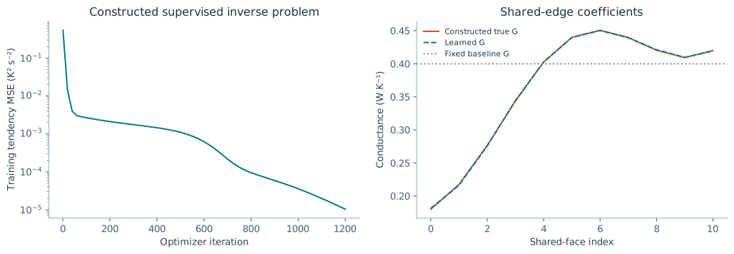
The descriptor x varies from −1 to 1 across the eleven faces. Each descriptor row is [x,x²,cos(πx)]. The constructed reference conductance is 0.25+0.12(x+1)+0.07cos(πx), in W K⁻¹. This rule is published so that the inverse-model experiment is exactly specified; it is not inferred from observations. Training temperatures are independent normal perturbations of 285 K with a 3 K standard deviation. There are 192 constructed training fields and 96 new constructed test fields on the same graph.
The model minimises mean squared node-tendency error. It does not receive the true G array as a supervised label. However, the target tendencies are generated by the same class of diffusion operator used by the learner. That makes the task useful for checking optimisation and identifiability within a controlled model class, and correspondingly weak as evidence about real-world transfer. The exact gradient is derived in Paper 4; the source computes it manually in NumPy and checks selected entries using centred finite differences.
Adam is implemented with fixed β₁=0.9, β₂=0.999, learning rate 0.015 and denominator offset 10⁻⁸, for 1,200 full-batch steps with seed 23. The method reference is Kingma and Ba, Adam: A Method for Stochastic Optimization. No claim is made that these settings are optimal, and no hyperparameter selection using test outcomes is performed.
3. Numerical verification before interpretation
For pure diffusion, the Euler step is a convex combination when Δt≤minᵢCᵢ/ΣⱼGᵢⱼ. The browser control uses a fraction of that bound and recomputes it for each selected closure. Positivity of G guarantees neither a stable arbitrary time step nor the physical correctness of a diffusive closure. The source rejects time steps beyond the bound rather than silently clipping the updated state.
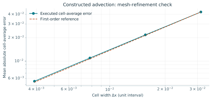
The source also checks a first-order periodic advection solver. The target is the exact cell average of a translated sinusoid, not an unrelated point sample. Four meshes use 32, 64, 128 and 256 cells over a unit interval with the same final time. This exposes the discretisation error while preserving the total conserved scalar. The finite-volume method reference is the Clawpack Riemann Book. The complete update, Courant number and manufactured solution are given in Paper 2.
Additional tests verify a minimum-change equality projection and its failure to enforce non-negative rainfall, and hand-calculated empirical versus fair CRPS. These deliberately small cases catch errors that a large model benchmark may not reveal. Equality projection uses a linear solve, not an explicitly computed inverse. The CRPS implementation rejects a one-member fair estimator and retains absolute-error behaviour for the one-member empirical distribution.
4. What actually ran
These values are generated from report.json, not written as expected outcomes. The held-out tendency test uses new constructed fields on the same graph and from the same distribution. The fixed-conductance baseline is G=0.4 W K⁻¹ for every edge; it is not a data-only neural competitor. The run therefore cannot measure the empirical benefit of conservation over an unconstrained network. Its conservation property is imposed by the update construction.
No real meteorological observations, satellite retrievals, NowcastNet weights, TimesFM checkpoint or WeatherNext issued predictions enter the executable experiment. No training on unseen geography, noisy observations or a different governing system is performed. All claims about model performance are restricted to the recorded constructed tendency problem. All source files, learned weights and diagnostics are downloadable for inspection.
| Artifact | Purpose |
|---|---|
| Python source | Full training, gradients, solver and assertions. |
| Learned weights | Archived MLP parameters used by the live browser view. |
| Training CSV | Recorded optimiser history; the last checkpoint is before its update. |
| Rollout CSV | Energy, step time, bounds and quadratic spread. |
| Conductance CSV | Constructed reference and learned edge coefficients. |
| Mesh-refinement CSV | Errors, Courant numbers and observed order. |
| SHA-256 manifest | Hashes of source, environment specification and numerical records. |
5. Reproduce, then extend
python -m pip install -r requirements.txt
python climate_math_lab.py --output results
The recorded environment is Python 3.12.14 and NumPy 2.3.5. The source needs NumPy only; no GPU or deep-learning framework is required for this small example. The notebook is a convenience entry point using the same functions. Its cells have not been separately executed in this update; the script execution and JSON report are the run record. Numerical results may differ slightly across environments, so checks use tolerances instead of bitwise output equality.
A useful next implementation stage changes one assumption at a time. First add observation noise and missing cells, then assess whether conductances remain identifiable from partial tendencies. Next test new geometry with dimensionless descriptors that have a physical interpretation. After those checks, add one physically justified source term and a separate source ledger. Only then combine the interface with real data adapters and a matched forecasting benchmark. This sequence keeps modelling errors distinguishable from optimisation or indexing errors.
For the climate thesis, a minimal real-data adapter should return field values, valid times, issue or availability times, units, spatial support, masks and provenance. A separate observation operator maps model states to the measured support. Every experiment should freeze training, validation and test events, preprocessing fits, grid geometry and code revision. A larger neural network does not remove these requirements. The dataset and interface contracts are part of the model definition.
6. From the development model to moist atmospheric dynamics
The heat experiment has a deliberately narrow state. A proposed atmospheric extension should first declare a single consistent state vector, not attach independent visual effects to each cell. One possible physical-coordinate starting point is a compressible, rotating, single-velocity moist mixture with fixed control volumes. The equations below are a proposed reference contract; they are not integrated by this development laboratory. Terrain-following coordinates and operational atmospheric formulations require additional metric and closure choices; see the WRF Version 4 technical note.
Mass conservation defines how density changes under transport. The momentum flux includes both movement of momentum and pressure forces across faces. Stress has the opposite sign inside this outward flux convention. Coriolis acceleration changes momentum direction; its instantaneous work is zero because u·(Ω×u)=0. Effective gravity and rotational conventions must be fixed consistently so the centrifugal contribution is not applied twice.
This total-energy statement differs from the earlier reduced sensible-heat ledger. Pressure work is already contained in the energy flux. Phase-dependent internal energy must be defined together with the equation of state and water-species variables. If latent reference energies are included in e, phase conversion and temperature recovery need a thermodynamically consistent treatment. Adding an independent latent-heating term without checking that convention can double count the same conversion. A temperature-only model cannot establish total moist-energy closure.
For example, a conversion rate C from water vapour to suspended liquid gives Sᵥ=−C and Sₗ=+C, in a two-phase conversion substep. The combined water mass does not change during that conversion. The temperature can change because the internal-energy partition changes. Precipitation reaching the ground is different: a complete formulation must represent a relative sedimentation flux and its boundary outflow, with corresponding mass, momentum and energy accounting. The displayed single-velocity equations alone do not produce falling rain.
Column water connects the state to surface precipitation
Let W=∫ρqₜ dz be total column water in kg m⁻² and let Mₕ=∫ρqₜuₕ dz be horizontal water transport in kg m⁻¹ s⁻¹. Under a declared impermeable upper boundary, consistent surface evaporation Eₛ and precipitation outflow Pₛ give the following column budget. Phase-conversion terms cancel when all water reservoirs are included. Side-boundary transport remains in the horizontal divergence.
For an assumed liquid-water density of 1,000 kg m⁻³, a surface mass flux Pₛ corresponds to 3,600Pₛ mm h⁻¹. This follows from converting mass per area to water depth and then seconds to hours. The conversion does not make a radar-reflectivity or rain-rate image a conserved water-density field. An observation operator and retrieval assumptions are still required to connect imagery to the model state.
The development modules must preserve this state contract
Represent each cell with extensive masses, momenta and energy. Use one shared vector of numerical fluxes per face; apply opposite signs to its two cells. Recover diagnostic temperature and pressure using the chosen thermodynamic relations. Couple phase conversion, boundary precipitation and surface exchange through explicit ledgers. Reject negative density, inadmissible species fractions or inconsistent thermodynamic states before they propagate into the next update.
A compressible solver also introduces acoustic wave speeds. A diagnostic time scale is cell width divided by |u|+c, where c is the relevant sound speed. The precise multidimensional stability bound depends on the numerical flux, time integrator and treatment of source terms; the heat model’s capacity bound cannot be reused as a general atmospheric time-step guarantee. Manufactured solutions, wave propagation tests, hydrostatic-balance checks and moist thermodynamic tests should precede a real-data forecasting benchmark.
Learned components can then target one declared closure, such as a transport coefficient or a constrained local conversion rate. Preserve the required source sums, dimensional units and positivity conditions. A lower residual for an incomplete equation does not establish better climate dynamics. The immediate development output here remains the executed heat-graph companion; the moist system is a specification for subsequent implementation and evaluation.
7. Research boundary and development decisions
The mathematics establishes conditional statements: paired internal exchanges cancel; a particular positive diffusion update has a sufficient convexity step bound; a compatible equality projection satisfies its constraints; a particular scalar stochastic process has a stated variance. None of these identities establishes that an atmospheric forecast will improve. The constructed training run shows that this implementation can fit a known class of tendencies and preserve the designed budget.
The proposed Caribbean system still needs chosen moist governing approximations, boundary and surface terms, independent observational evaluation, strong baselines and a defined forecasting horizon. Noise and model discrepancy can make a physically constrained inverse problem non-identifiable. A useful benchmark must expose those failure modes rather than suppress them with source terms or an overly strong prior. The six paper appendices specify these questions in greater mathematical detail.
This laboratory and the accompanying prose are AI-assisted development drafts attributed to Adrian Dunkley for review. No journal acceptance, thesis approval or institutional endorsement is asserted. All references are method sources, not evidence that the constructed experiment has been independently validated. The existing animations at the top of the paper series remain explanatory views; the new browser laboratory alone explicitly evaluates the archived learned conductance model.
Compare a reference and an estimate

The left specimen is fixed at 0.60 constructed unit.