Foundation priors and physics constraints: the Jamaican temperature experiment

Compare candidate trajectories. Filled isometric scientific teaching instrument. Each cartridge represents a candidate trajectory on the same comparison window. A valid comparison needs matched information, issue times and independently assessed targets. — Constructed explanatory instrument; it is not an observed atmospheric field or a trained-model result. Geometry uses Anatomy (MIT). The paper states its evidence and limits.

Research papers · Reformatted 31 Oct 2026Executed experiments and negative results ↗Theories and hypotheses ↗

Abstract

We formulate the integration of frozen foundation forecasts, local neural corrections and physical penalties, and report the executed Jamaican daily-temperature component experiment. The 2026 constrained PINN ensemble obtains 0.501669 °C MAE over 798 gridded site–lead targets, improving on AR(14) but remaining behind TimesFM 2.5 at 0.494714 °C. The full physics loss improves its matched graph network in 2026; the pooled effect is uncertain. Satellite augmentation and added context do not reliably improve generalisation. The targets are ERA5-derived grid cells, and historical evaluation is exploratory. These findings delimit the proposed moist space–time model rather than validating it.

Keywords: TimesFM; WeatherNext; foundation models; data assimilation; local forecasting

Thesis connection. This supplies actual component evidence on foundation priors, satellite inputs and a reduced physical closure. It constrains expectations for the proposed reconstruction. Read the hypotheses.

1. Distinct model roles and forecasting horizons

A temporal foundation model and a spatial weather model solve different prediction problems. TimesFM was introduced as a pretrained decoder-based model with patching for time-series forecasting. [1] It can supply a baseline for a declared local series, but an extracted temperature or rainfall trajectory does not encode a complete atmospheric state. A weather-model forecast can provide spatial context, yet its grid and output variables still need a mapping to local quantities.

WeatherNext documentation is a living source and must be cited with the generation and product actually used. [2] This paper does not label a fixed generation as the permanently latest model. A reproducible experiment should archive the issue time, valid times, product identifier, model generation, variables, spatial support, licence and access method. If an intended model or historical forecast archive is unavailable, it should remain an unexecuted comparator rather than being replaced with an unlabeled surrogate.

2. Priors, observations and a constrained local state

Let f₀ provide a prior local forecast derived from available context, and let H map the local state to observations. A local correction can fit available observations while being penalized for departure from both the prior and selected physical constraints. This resembles established estimation and assimilation ideas; the presence of a neural prior alone is not a sufficient novelty claim. The distinguishing research question concerns the effects of a particular prior and constraint under controlled information access.

\mathbf{x}^{*} = \operatorname{arg} \operatorname{min}_{x} { \|H(\mathbf{x}) - \mathbf{y}\|_{R^{-1}}^{2} + \|\mathbf{x} - \mathbf{f}_{0}\|_{P^{-1}}^{2} + \lambda \|\mathcal C(\mathbf{x})\|^{2} }

(1)

R and P represent chosen observation-error and prior-error covariance models; C is a scaled physical residual. Invertibility or regularization must be specified.

This expression is a proposed estimation objective, not an executed training result. If the larger model and the local observations share information through an upstream analysis, errors may be correlated. Treating P and R as independent diagonal matrices is a modelling assumption, not an empirical fact. Covariance sensitivity should therefore form part of the benchmark, especially when a strong prior suppresses local extremes.

A residual correction should also preserve the distinction between analysis and forecast. At issue time, available observations may update the initial state. Future observations may evaluate the forecast but cannot enter that initial correction. A retrospective reconstruction that uses future observations must be labelled smoothing or reconstruction rather than an operational forecast.

3. An analytical example of uncertainty growth

Consider a scalar anomaly driven by linear relaxation and additive stochastic forcing. This is a tractable demonstration of uncertainty evolution, not a model of Jamaican rainfall. With damping a>0 and driving-noise amplitude σ, the variance has a closed-form solution. It shows why a forecast interval should depend on lead time and process assumptions rather than being drawn as a decorative cone.

dX = -aX dt + \sigma dW_{t}

(2)

X: scalar anomaly; a: damping (h⁻¹); σ: driving-noise amplitude (anomaly units h⁻¹ᐟ²); W: Wiener process with time measured in hours.

\operatorname{Var}[X(t)] = V_{0}e^{-2at} + \frac{\sigma ^{2}}{2a}(1 - e^{-2at})

(3)

Assumes a linear scalar system and independent initial uncertainty. For a=0, the limit is V₀+σ²t.

Figure 1. Analytical anomaly standard deviation for V₀=0.25 K², σ=1 K h⁻¹ᐟ² and damping a=0, 0.1 and 0.3 h⁻¹. These curves are not model-performance or atmospheric validation results. Download figure data (CSV).

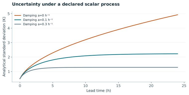
A larger ensemble spread is not automatically better or worse. Calibration asks whether forecast distributions match observed frequencies; sharpness concerns concentration, conditional on calibration. Proper scoring rules provide a principled way to assess probabilistic predictions. [4] The analytical interval here satisfies its constructed assumptions and says nothing by itself about the calibration of a real weather model.

4. Benchmark and physics ablation

Use one frozen target archive and identical forecast cutoffs. Compare seasonal or diurnal climatology, persistence, a conventional statistical model, a pinned TimesFM checkpoint, accessible issued larger-scale weather forecasts and local correction variants. Include the direct coarse-to-local mapping as a baseline; otherwise any improvement may simply reflect spatial adaptation. For each model, record input history, missingness handling, preprocessing fits and compute budget.

Separate the information ablation from the physics ablation. First, hold the correction architecture fixed and add or remove the larger-scale prior. Second, hold inputs and architecture fixed while changing the physical constraint. Third, assess the interaction of both additions. This factorial comparison can show whether physics helps only when the prior is weak, or whether prior information accounts for most apparent improvement. Fit all scaling and calibration using training or validation data.

GraphCast is a relevant learned weather-model precedent, but its published global task differs from a local Caribbean rainfall target. [3] Lead-time curves should therefore compare models only on matched variables, valid times and supports. A global model’s aggregate benchmark ranking is not a substitute for this experiment.

5. Failure modes and attribution

Inspect performance by lead time, rapid-change events, terrain exposure and input age. A forecast can remain close to its prior while missing local transitions. Conversely, an unconstrained correction can fit local observations and then drift during rollout. Report both behaviours and examine whether constraints suppress physically meaningful extremes. A poorly chosen physical residual may encode an approximation error as a strong penalty.

Feature attribution should be interpreted within the model and dependence structure. Permuting a satellite predictor while leaving correlated variables unchanged can produce an unrealistic input. A more informative analysis combines controlled variable removal, delayed-input tests and physical perturbations with clear constraints. Any saliency or feature-importance graphic should be labelled as a diagnostic association rather than a causal explanation.

6. Contribution and implementation status

The executed component study now supplies the comparison that the earlier protocol required. Section 8 reports actual archived TimesFM, local-network, satellite and WeatherNext outcomes. The present website revision independently recounts saved primary scores; it does not rerun foundation inference or refit the neural models. The central empirical limitation is that the full PINN and its constrained ensemble do not uniformly improve on strong frozen comparators.

The formal estimation objective and scalar uncertainty example remain separate methodological constructions. They are not the objective or calibration model used to generate every archived forecast. The next real-atmosphere step is a moisture-reconstruction benchmark with matched observation windows, boundary information, withheld data and compute. A hydrostatic neural field, a local daily-temperature graph and a nowcasting generator have different state variables and cannot serve as interchangeable evidence.

7. Mathematical derivation and development

7.1 Deriving a Gaussian analysis update

Let the background forecast x_b have a chosen Gaussian error covariance P, and let observations have covariance R under a linear operator H. Assume these errors are independent for this derivation. Minimising the sum of background and observation quadratic terms gives a stationarity equation. Collecting the coefficients of x yields a linear system with a positive-definite Hessian when P and R are positive definite. Correlated background and observation errors require an altered joint model.

(P^{-1} + H^{T}R^{-1}H)\mathbf{x}_{a} = P^{-1}\mathbf{x}_{b} + H^{T}R^{-1}\mathbf{y}

(A1)

Derived by differentiating the stated quadratic objective. x_a is an analysis, not a future forecast and not a claim that a foundation model is calibrated.

\mathbf{x}_{a} = \mathbf{x}_{b} + K(\mathbf{y}-H\mathbf{x}_{b}) ; K = PH^{T}(HPH^{T}+R)^{-1}

(A2)

Equivalent gain form under the same invertibility assumptions. Use linear solves for implementation.

Worked example

For one constructed temperature, let the background be 28 °C with variance 4 K² and the observation be 30 °C with variance 1 K². With H=1, K=4/(4+1)=0.8 and the analysis is 29.6 °C. The posterior variance in this assumed Gaussian model is (1−K)P=0.8 K². This is a conditional calculation under stated covariances, not an estimated uncertainty for Jamaica.

This example shows why a numerical weight must be linked to uncertainty and support. An apparently precise observation can dominate an analysis even if it is a biased retrieval or an inappropriate local surrogate. P and R should be estimated or sensitivity-tested using training and validation information. They cannot be tuned on the final test events and then described as independently calibrated.

7.2 Physical residuals and differentiable corrections

Add a residual vector c(x), scaled into dimensionless physical components, to the objective. For a squared residual penalty ½λcᵀc, the gradient contribution is λJ_cᵀc. A Gauss–Newton approximation adds λJ_cᵀJ_c to the background-plus-observation Hessian. This approximation neglects second-derivative terms weighted by the residual itself. It is a numerical choice that should be checked when the residual is large or the physics is strongly nonlinear.

g = P^{-1}(x-x_{b}) + H^{T}R^{-1}(Hx-y) + \lambda J_{c}^{T}c(x)

(A3)

Gradient of a half-weighted quadratic objective; the factor convention differs from an objective written without the one-half factors.

A_{GN} = P^{-1} + H^{T}R^{-1}H + \lambda J_{c}^{T}J_{c} ; A_{GN}\delta x = -g

(A4)

Gauss–Newton direction. A line search or trust-region strategy may be needed; one iteration is not guaranteed to solve the nonlinear estimation problem.

If c is a discretised physical tendency, record exactly which variables and boundary data enter it. A mismatch between a coarse prior and a local boundary operator can create an irreducible residual. Increasing λ then forces a compromise with the data, not necessarily a more accurate atmosphere. A hard equality projection and a soft penalty answer different questions and should remain separate ablations.

7.3 Backpropagating a multi-step physical rollout

Let a learned update be x_{k+1}=Φθ(x_k,u_k), where u_k denotes available forcing. Training only on one-step errors can leave accumulation of state-dependent errors untested. A rollout loss includes errors at multiple leads, with the target and its availability rules fixed in advance. Differentiation through repeated updates requires the chain rule through every intermediate state; detaching those states changes the objective.

S_{k+1} = J_{x}\Phi _{\theta } S_{k} + J_{\theta }\Phi _{\theta } ; S_{0} = 0

(A5)

Forward sensitivity of rollout state to parameters when the initial state is fixed. A learned or assimilated initial state changes S₀.

A reverse-mode implementation accumulates the same dependencies in the opposite computational direction. Standard automatic differentiation frameworks expose this computational graph, as described by the PyTorch autograd documentation. [5] The NumPy companion implements an explicit single-step gradient so that the derivative can be inspected independently; it does not execute a foundation model or claim multi-step neural training. Long atmospheric rollouts may require checkpointing, shorter training segments and stability controls. Those are development decisions to benchmark rather than assumed guarantees.

7.4 Forecast uncertainty and the analytical scalar example

For the scalar process dX=−aXdt+σdW, the integrating factor gives X(t)=e⁻ᵃᵗX(0)+σ∫₀ᵗe⁻ᵃ⁽ᵗ⁻ˢ⁾dW(s). The first term carries initial uncertainty, and the second introduces process uncertainty. Assuming the initial state is independent of the future noise, the cross covariance is zero. Applying the variance rule for the stochastic integral yields the expression used in the animation.

V(t) = e^{-2at}V_{0} + \sigma ^{2}\int _{0}^{t}e^{-2a(t-s)}ds = e^{-2at}V_{0} + \frac{\sigma ^{2}}{2a}(1-e^{-2at})

(A6)

For a>0. The a→0 limit is V₀+σ²t. The implementation uses expm1 to avoid cancellation for small damping.

The finite long-lead variance is a consequence of positive damping in this chosen scalar model. It is not a general bound on atmospheric uncertainty. Likewise, an interval based on 1.96 standard deviations has its stated marginal interpretation only under the Gaussian assumptions of this example. Real forecast calibration requires observed outcomes and a proper evaluation procedure.

7.5 Development contract for foundation-model integration

Create a versioned forecast adapter with issue_time, valid_time, variable, units, grid and availability fields. Reject predictors arriving after the declared cutoff.
Map the coarse forecast to local support before the correction stage. Archive that direct mapping as a baseline.
Fit a statistical correction, a neural correction and a constrained correction with the same observation access. Keep prior-information and physics ablations separate.
Evaluate complete withheld events and lead-time curves. Identify when an updated analysis is being compared with a genuine forecast.

TimesFM can be an explicitly pinned time-series baseline, while an accessible WeatherNext product can provide versioned spatial context. Neither is executed in this development companion. A local posterior calculation or a stable scalar uncertainty animation cannot establish either model’s local skill. The required next step remains an accessible issued-forecast archive and an independent observational benchmark.

8. Recorded Jamaican temperature experiment

Source: Dunkley, Jamaica Temperature Forecasting: Technical Report and Model Comparisons, 14 October 2026, and its archived research package. These are author research records, not peer-reviewed external findings. The online edition independently recounts 3,520 primary MAE/RMSE rows from saved predictions. Models were not retrained for this edition.

Targets are ERA5-derived daily mean 2 m air temperatures returned by Open-Meteo, with elevation adjustment disabled. The six air cells provide coarse regional support; the labels Kingston, Montego Bay and Mandeville do not identify station measurements. NASA POWER/CERES radiation and cloud fields are coarser still. Two NOAA OISST points supply ocean temperature, not sea level. Image pixels displayed for geography were not model inputs. The archive has 6,117 daily records per air cell, 1 January 2010–30 September 2026. Spatially duplicated radiation histories and 61 carried-forward tail days are retained in the source audit.

The current outer period comprises 192 weekly origins and 4,032 site–lead targets in 2023–September 2026. The 2026 subset comprises 38 origins and 798 targets. Each origin predicts seven days at three target cells; dates are scored chronologically. Earlier research rounds inspected overlapping historical periods, so these are exploratory evaluations. Imposed seven-day radiation and fourteen-day SST lags restrict the information set but do not prove historical product-release availability.

Model	2026 MAE (°C)	2023–2026 MAE (°C)
TimesFM 2.5	0.494714	0.498389
AR14 traditional	0.534926	0.516715
Graph NN satellite	0.525773	0.525415
Graph PINN full	0.514202	0.519533
PINN ensemble	0.501669	0.496632

The constrained PINN ensemble reduces 2026 MAE by 6.22% relative to AR(14), but is 1.41% worse than TimesFM 2.5. The full graph PINN improves its matched satellite graph network by 2.20% in that year. For the pooled period, the four-week paired block interval for full PINN minus matched graph NN is [−0.01332, 0.00181] °C; it includes zero. Its physics term is therefore not evidence of a uniform, independently confirmed improvement.

Interactive scores and archived forecast cases. Change period, location and origin; the designated failure case is selected by worst full-PINN 2026 origin error, rather than presented as a random example. Full metric table.

Recorded 2026 MAE against the same ERA5-derived targets. No station-validation claim.

Worst 2026 full-PINN origin across sites and leads; the Mandeville-labelled cell is shown. Selection is explicit, not a random representative case.

Satellite augmentation and additional context cells do not reliably improve generalisation. The worst full-PINN origin is 26 January 2026: all displayed local models miss the late-window cooling. Synoptic transport is a plausible missing mechanism, but the dataset does not identify the event’s cause. Actual WeatherNext 2 and ECMWF IFS fixed-lead archive fields overlap on 16 weekly origins. Those daily aggregates are not a verified single-initialisation trajectory. A post hoc eight-week calibration/eight-week scoring diagnostic reduces WeatherNext bias, while its fixed blend still loses to TimesFM on the scoring subset.

Source audit · Paired intervals · Independent recount receipt

9. The executed local neural model

The archived satellite experiment uses a shared 77 → 16 → 16 → 7 network with two tanh hidden layers. The 77 predictors comprise 26 temperature, radiation and calendar entries; 22 satellite radiation/cloud entries; eight SST entries; and three seven-day forecast vectors. Local corrections are bounded to ±2 °C by the final tanh. These are actual component-model dimensions, distinct from the proposed coordinate-conditioned atmospheric field.

\mathbf z_i^{(1)}=\tanh(W_1\mathbf c_i+\mathbf b_1),\quad\mathbf z_i=\tanh(W_2\mathbf z_i^{(1)}+\mathbf b_2),\quad\boldsymbol\delta_i=2\tanh(W_3\mathbf z_i+\mathbf b_3).

(B1)

Input scaling is fitted on the allowed training information. The local output contains seven lead-specific temperature corrections in °C.

A symmetric distance-based graph weights a learned sigmoid conductance. The normalisation uses the maximum row sum, rather than separately normalising each row, so symmetry is retained. With approximate horizontal distance D in kilometres:

A_{ij}=e^{-D_{ij}/100}\mathbf1_{i\ne j},\quad W_{ij}=\frac{A_{ij}}{\max_k\sum_l A_{kl}},\quad c_{ij}=0.15W_{ij}\,\sigma(\mathbf w^T|\mathbf z_i-\mathbf z_j|+b).

(B2)

c is symmetric, non-negative, and has row sums at most 0.15. It is a dimensionless daily anomaly-exchange coefficient, not a measured atmospheric heat conductance.

e_{i,h}=\sum_jc_{ij}(u_{j,h-1}-u_{i,h-1}),\qquad \sum_i e_{i,h}=0.

(B3)

Pairwise cancellation conserves the sum of anomaly increments under equal implicit capacities. It is not a physical atmospheric energy budget.

The recursive update adds changes in a base forecast and bounded local correction, then the exchange. The physical penalty compares this forecast with a phenomenological relaxation, radiation and SST closure. Its coefficients and uncertainty are model assumptions. Matched graph controls use the same inputs, scaling, architecture and seed count. The recorded outcomes therefore test one reduced regulariser; they do not prove moisture or momentum dynamics.

References

AI-assisted drafting and implementation. Author and supervisory review are required before submission. The source-reported rainfall campaign, independently recounted temperature scores and constructed numerical laboratory have distinct evidence scopes.

References

- [1] Das, A., Kong, Sen & Zhou (2024). A decoder-only foundation model for time-series forecasting. Proceedings of ICML, PMLR 235, 10148–10167.
- [2] Google. WeatherNext model documentation. Living documentation: record the model generation, issue time, licence and dataset version for each experiment.
- [3] Lam et al. (2023). Learning skillful medium-range global weather forecasting. Science, 382, 1416–1421.
- [4] Gneiting & Raftery (2007). Strictly Proper Scoring Rules, Prediction, and Estimation. Journal of the American Statistical Association, 102, 359–378.
- [5] PyTorch documentation. Autograd mechanics. Versioned documentation inspected for computational-graph semantics.