Inspect a sampled field

The carriage represents an observation with a particular footprint.
Abstract
We examine observation support, conservation and identifiability in rainfall downscaling, and connect the derivation to the recorded Jamaican CHIRPS component campaign. A hard aggregate constraint improves the matched neural learner, while seasonal allocation remains more accurate in the listed within-product tests. Artificial driver perturbations expose inherited parent-mean error. The formal treatment separates representation spacing from independently supported information and defines the additional evidence required for atmospheric moisture reconstruction. The recorded rainfall outcomes are source-reported retrospective component results; they do not establish month-ahead forecasting or a full atmospheric PINN.
Keywords: downscaling; IMERG; CHIRPS; observation operator; identifiability; Jamaica
Thesis connection. This tests the aggregate-constraint component and its sensitivity to coarse-driver error, corresponding to hypothesis H1. Read the hypotheses.
1. Why spatial support matters
A satellite retrieval, a station gauge and a model cell refer to different spatial and temporal supports. Comparing them as if they were interchangeable point measurements confounds representation error with forecast error. This distinction is central to DLEGOS: a one-kilometre computational cell can receive information from a much larger meteorological grid, but the interpolation does not create a new independent observation.
The NASA IMERG Version 07 documentation describes combined precipitation estimates on half-hourly 0.1° × 0.1° fields. [1] The original CHIRPS record combines satellite information and stations for a long rainfall record at 0.05° support, including daily products. [2] These are distinct observing products, not interchangeable labels for rainfall truth. Product versions, accumulation conventions and availability times should be fixed in an experiment manifest.
2. The observation operator
Let x denote the local state vector and y a product value. The observation operator H maps local states to the product’s support, while ε includes retrieval, measurement and representation uncertainty. For an areal mean, H should weight by actual overlap area and respect missing or masked cells. For a point gauge, the operator and uncertainty differ. A single bilinear interpolation rule is not an adequate universal description.
For accumulated precipitation, temporal support is as important as spatial support. A half-hour mean rain rate is not a known within-window sequence. Converting rate to depth requires multiplication by interval duration; converting a daily depth into hourly rates requires an additional assumption and must not be described as observed hourly evolution. Time stamps must identify whether they denote the beginning, centre or end of the accumulation period.
Operational evaluation adds another axis: availability. A retrospective final product may improve the target archive but leak future information if used as an issue-time predictor. Each input record therefore needs both valid time and earliest practical availability. A delay-sensitivity experiment can distinguish the benefits of a better observation from the benefits of information that would not yet have existed.
3. Conservative allocation and its null space
For one coarse footprint with mean rainfall R̄, assign each local cell a positive score wᵢ. Normalize these scores using overlap areas Aᵢ. The resulting cell values preserve the prescribed coarse mean by construction. Positivity can be enforced by choosing wᵢ = exp(zᵢ), with a numerically stable softmax implementation.
This constraint does not identify the fine field. With m local cells and one independent coarse mean, there are generally m−1 unconstrained directions before additional observations or priors are imposed. For equal areas, adding a perturbation vector whose entries sum to zero preserves the mean. Terrain, land cover and learned spatial priors may select one allocation, but the selected pattern remains a model inference. Coarse agreement cannot independently validate that selection.
4. Interactive allocation and an explicit counterexample
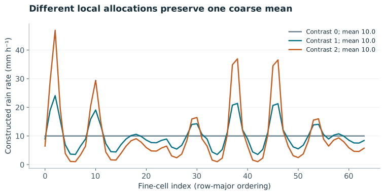
The zero-contrast case allocates equal rainfall to every cell. Increasing contrast produces pronounced local extremes while retaining the same coarse total. Neither extreme pattern is established as correct by the coarse observation. This counterexample is the practical reason to avoid describing a detailed visualization as high-resolution evidence. The appropriate claim is that the allocation satisfies a specified aggregate constraint.
5. Study design for Jamaica
A proposed Jamaican experiment should compare a constant-footprint allocation, a terrain-based statistical model, an unconstrained learned model and a conservative learned model. Keep predictors and training events aligned. Evaluate coarse consistency separately from station error. Withheld gauges must not have been directly included in the training target or indirectly blended into the same target product without disclosure; otherwise the apparent independence of verification is weakened.
Partition complete periods and locations, and maintain the same masked domain across models. Report rain occurrence and conditional intensity separately so that improved wet-day detection does not obscure intensity bias. For terrain effects, test altitude and exposure strata only when the observational sample can support them. Include a coarse-input perturbation experiment: a perfectly conservative allocator can preserve an erroneous input total and thereby transmit its bias to every local solution.
The existing NASA POWER regional inputs provide a useful contrast with the detailed terrain mesh. [3] They show how fine geometry and coarse meteorology can coexist without implying locally observed forcing. Those inputs should remain provenance-labelled, and should not be recast as an independent local rainfall validation dataset.
6. What the thesis can claim
The mathematical claim is that a normalized positive allocation can preserve an imposed coarse mean. The scientific claim that the fine allocation improves local rainfall prediction requires withheld information at an appropriate support. These claims should be evaluated and reported independently. A constrained model that retains coarse bias or misses local extremes is not rescued by its exact aggregate identity.
This paper supplies the observation model needed by subsequent DLEGOS experiments. Its next empirical step is a versioned, quality-controlled pairing of retrieval footprints and independent local observations. The fine-grid demonstration is executable but illustrative. No satellite rainfall reconstruction, station-fitted downscaler or new product-validation result is asserted here.
7. Mathematical derivation and development
7.1 Constructing the spatial observation operator
Let fine cell i have area Aᵢ, and let observation footprint k overlap it over area aₖᵢ. For a valid areal mean, Hₖᵢ = aₖᵢ/Σⱼaₖⱼ. Each supported row sums to one and produces a mean in the same units as the local field. A total-depth or volume observation needs a different operator and dimensional conversion. Missing or ocean-masked cells alter both the support and the normalization; replacing missing values by zero is a substantive assumption.
For geographic grids, use actual cell overlap areas or a justified spherical approximation. A row that sums to one is necessary for constant-field preservation but does not prove its geography is correct. Test the operator on a constant field, an isolated impulse and a simple spatial gradient. These tests detect support and indexing errors before a neural downscaler can obscure them. Temporal accumulation needs an analogous operator so that a daily depth is not silently compared with an instantaneous rate.
7.2 Rank, null spaces and unresolved degrees of freedom
Stacking observations gives y = Hx + ε. In the noiseless compatible case, every solution can be written as one particular solution plus a vector in the null space of H. The dimension of that null space is n−rank(H). Consequently, one coarse mean over n fine cells cannot identify all fine-cell values, even if a rendering displays them separately. A spatial prior supplies a preference over the unresolved degrees of freedom; it does not turn them into observed quantities.
Four equal-area cells with values [3,5,7,9] have mean 6. The perturbation [1,−1,2,−2] has zero mean, so [4,4,9,7] produces the same coarse observation. Both fields are non-negative and agree exactly with the coarse input; the observation cannot select between their local patterns.
7.3 Deriving a minimum-change equality projection
Suppose a network first produces a provisional fine field z. One way to impose compatible coarse observations b is to change z as little as possible in a declared quadratic metric. Let P be a positive-definite correction covariance or weighting matrix. Minimise one half of (x−z)ᵀP⁻¹(x−z), subject to Hx=b. Introduce a multiplier λ and differentiate the Lagrangian with respect to x. This yields x−z = PHᵀλ. Substitute back into the equality to obtain a much smaller system for λ.
The derivation also shows exactly what the projection guarantees: the imposed linear equalities, to the numerical solver tolerance. It does not guarantee non-negative rainfall. With P=I, one equal-area mean constraint and z=[2,4,6,8], the mean is 5. A target mean of 6 adds one to each cell, giving [3,5,7,9]. A target mean of zero instead subtracts five and gives [−3,−1,1,3]. The equality holds but the field is physically inadmissible for rainfall.
residual = b - H @ z
multiplier = np.linalg.solve(H @ P @ H.T, residual)
x = z + P @ H.T @ multiplier
7.4 Non-negativity, overlapping footprints and noise
For rainfall, combine equalities with x≥0 in a constrained quadratic programme, or choose a positive parameterisation with a constraint mechanism that actually matches the supports. Independent softmax normalization works for a disjoint partition with one declared coarse mean per footprint. It does not generally satisfy several overlapping footprints simultaneously. Repeatedly normalising one footprint can break the constraint previously imposed on another. State this limitation before using the single-footprint formula in a multi-sensor setting.
If b contains noisy or mutually inconsistent retrievals, enforcing Hx=b exactly can be inappropriate or impossible. A soft likelihood term uses an error covariance R and allows residuals according to uncertainty. The covariance should include shared retrieval or station-blending information where it matters. If H is rank-deficient, a pseudo-inverse can define one minimum-norm correction, but it cannot make an incompatible target compatible. Examine the residual and report the effective rank.
7.5 Differentiating the correction and designing the test
With fixed H and P, the equality projection is affine in z. Its Jacobian is I−PHᵀ(HPHᵀ)⁻¹H. Multiplying that Jacobian by H yields zero, so a first-order change in the provisional field remains within the equality constraint after projection. This is useful for training a network through the projection. If H or P depends on learned parameters, their derivatives must also be included; treating them as constants changes the optimisation problem.
The development companion verifies the equality and includes the negative-rainfall counterexample. A subsequent downscaling study should assess coarse residuals and independent fine-support error separately, with the observation operator frozen across alternatives. Deliberately perturb coarse totals to measure transmitted input bias. Test footprint overlaps and missing masks before claiming a multi-sensor conservative downscaler. No station-fitted or satellite-validated rainfall model is trained by this companion.
8. Recorded Jamaican rainfall component studies
The 6 October 2026 execution assessment reports 51 trained neural models: 45 primary fits and six longer-training diagnostics. The task is conditional spatial reconstruction using the observed target-month coarse rainfall. It is not a month-ahead forecast. The hard output normalises positive allocations to conserve the supplied area-weighted parent depth. This is an aggregate precipitation-volume constraint, distinct from atmospheric moisture-budget closure.
| Training setting | Free network | Hard network | Seasonal allocation |
|---|---|---|---|
| 18 years; 200 epochs | 15.36 | 14.23 | 9.73 |
| 18 years; 1,000 epochs* | 13.52 | 12.57 | 9.73 |
| 3 years; 200 epochs | 17.77 | 16.43 | 9.61 |
| 1 year; 200 epochs | 20.79 | 19.07 | 11.38 |
Area-weighted test RMSE in mm/month against 2022–2025 CHIRPS fields; neural ensembles average seeds 11, 29 and 47. *The 1,000-epoch runs were post-score diagnostics. The primary hard-minus-free difference is −1.14 mm/month, with a source-reported paired 12-month-block interval [−1.43, −0.76]. The hard model is 4.49 mm/month worse than seasonal allocation, with interval [2.45, 6.28]. Rounded table values need not subtract to the separately computed unrounded difference.
Official monthly CHIRPS v2 rasters span 2000–2025. The retained geometry has 360 cells in 29 non-overlapping 0.20° parents, using native 0.05° fields. Training, validation and test contain 216, 48 and 48 months. The test has 17,280 cell-months, but resampling keeps entire fields together. Nine irregular Sangster airport test months pass the complete-daily-record screen; no Norman Manley test month qualifies. Those point-versus-grid comparisons do not support national ground-truth claims. Their ranking differs from the primary CHIRPS comparison.
Artificial ±20% coarse-driver scaling gives a reported aggregation-error RMSE floor of 31.67 mm/month; hard-model errors are 35.27 and 34.87. These are declared interventions, not measured biases of a forecast system. Substituting a training-seasonal coarse driver gives 84.49 mm/month RMSE, and a previous-year same-month driver gives 109.84. The network was frozen: those substitutions expose dependence on the supplied driver and are not comparisons between separately optimised forecast models.
Source: Dunkley, Jamaican physics-informed rainfall experiments: Execution, scientific assessment and literature update, 6 October 2026, pp. 1–3. Numbers in this section are source-reported; the rainfall training archive was not rerun in this website revision. The normalisation has established prior art in Harder et al., JMLR 24(365), 2023. [R040]
References
- [1] NASA GPM. IMERG Version 07 Technical Documentation. Product documentation; consult the selected run and version for latency and support.
- [2] Funk et al. (2015). The climate hazards infrared precipitation with stations—a new environmental record for monitoring extremes. Scientific Data, 2, 150066.
- [3] NASA POWER. Hourly point API: historical source response embedded in the DLEGOS workbench.