Conservative graph coupling for a cell-based atmospheric world model

Coordinate local numerical fields. Filled isometric scientific teaching instrument. Each station represents a numerical subdomain with an explicit physical state. Accounting, positivity, stability and state accuracy are different tests. — Constructed explanatory instrument; it is not an observed atmospheric field or a trained-model result. Geometry uses Anatomy (MIT). The paper states its evidence and limits.

Research papers · Reformatted 31 Oct 2026Executed experiments and negative results ↗Theories and hypotheses ↗

Abstract

This paper specifies a graph representation for the DLEGOS cell-based atmospheric world model. Nodes store local states and geometry, while edges represent physically declared shared interfaces. We distinguish learned information messages from transported physical quantities and derive a conservative update based on an oriented incidence matrix. The construction makes internal cancellation explicit even when a learned model supplies edge fluxes. A two-cell analytical example and an interactive spatial lattice illustrate the relationship between topology, coupling and time evolution. The framework remains a proposed architecture: a rotating lattice is a visualization, and a conservative heat exchange is not a complete atmospheric solver. The thesis contribution is an auditable interface specification and a set of tests that can separate graph expressivity, physical accounting and predictive usefulness.

Keywords: graph neural networks; finite volumes; fluxes; DLEGOS; world models

Thesis connection. This develops the local coupling mechanism to be tested under sparsity, corresponding to hypothesis H2. Read the hypotheses.

1. A cell plus a time history

DLEGOS uses “tesseract” to describe a spatial control volume together with its temporal trajectory. The graph at a fixed time contains the active atmospheric cells above terrain. A trajectory connects successive states of the same cell. Spatial edges and temporal dependencies therefore have distinct meanings. The website’s three-dimensional lattice is a spatial slice of this representation, not a numerical proof that time is reversible or that a literal four-dimensional hypercube is being integrated.

Graph-based learned weather prediction supplies a relevant architectural precedent; GraphCast demonstrates learned message passing for global forecasting. [1] That precedent motivates evaluating graph representations, but does not establish a novelty claim for DLEGOS or guarantee that an arbitrary message-passing layer conserves physical quantities. Novelty must be tied to the proposed interface constraints, observing conditions and tested outcomes.

2. State variables, geometry and physical meaning

Each node should distinguish prognostic quantities from diagnostics and prescribed inputs. A minimal heat experiment stores sensible-heat capacity and temperature; a moist atmospheric extension needs a thermodynamically consistent set of mass, momentum and energy variables. Pressure derived from a prescribed column differs from pressure evolved with a compressible dynamical core. The selected equations, coordinate system and approximations must be declared together. [2]

Each edge stores an orientation, shared face area, centre separation and boundary type. Terrain cells that do not share an open atmospheric face should not exchange a physical flux merely because their display cubes are nearby. Conversely, a learned information graph may use additional long-range edges. Such edges can convey context but should not silently become pathways for nonlocal mass transport. The architecture should maintain separate information and transport graphs when their semantics differ.

3. Incidence matrices and conservative learned fluxes

Choose one orientation for each internal edge. Let Bᵢₑ equal +1 at the receiving cell, −1 at the sending cell and zero elsewhere. Let qₑ be the extensive transfer rate in the chosen orientation. The update acts on the extensive stored quantity U, rather than applying equal temperature increments to unequal cells.

\mathbf{U}^{n+1} = \mathbf{U}^{n} + \Delta t (B\mathbf{q}^{n} + \mathbf{s}^{n})

(1)

For heat, U is energy in J, q is edge power in W and s is external heating in W. B is dimensionless.

\mathbf{1}^{T}B = \mathbf{0}^{T} ⇒ \mathbf{1}^{T}\Delta \mathbf{U} = \Delta t \mathbf{1}^{T}\mathbf{s}

(2)

Every internal edge has one positive and one negative incidence entry. Open boundary fluxes require separate columns or explicit source terms.

A neural edge function may produce qₑ from neighbouring states, geometry and available environmental context. Using the same predicted qₑ for both endpoints preserves cancellation. It does not guarantee stability, positivity, accurate constitutive behaviour or correct boundary forcing. Those are separate constraints and tests. For unequal capacities Cᵢ and Cⱼ, a transfer Q changes temperatures by Q/Cᵢ and −Q/Cⱼ, respectively; equal-and-opposite temperature increments would generally violate energy accounting.

A physics-informed residual can complement this structure, following the broader PINN approach, but the roles differ. [3] A residual asks whether the learned state obeys selected local equations. The incidence construction fixes how an internal transfer is booked. Combining them requires consistent operators and nondimensional scaling; simply adding more terms does not ensure a meaningful objective.

4. Interactive topology and temporal exchange

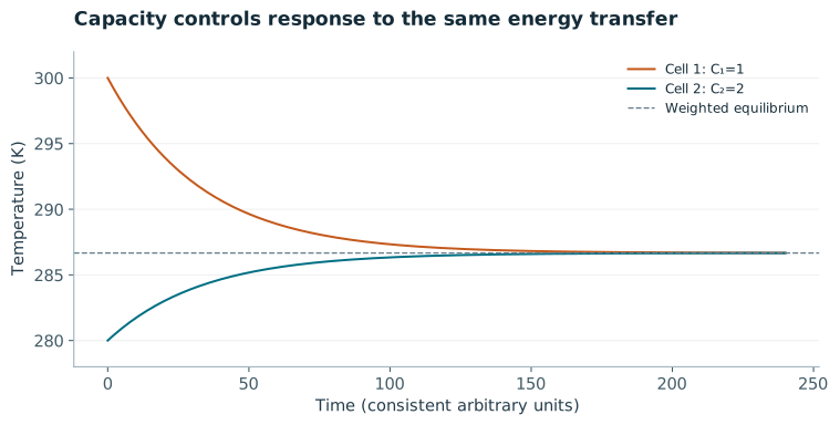
Figure 1. Exact unequal-capacity exchange: C₁=1, C₂=2 (consistent arbitrary energy-per-kelvin units), G=0.02, T₁=300 K and T₂=280 K. The equilibrium is 286.67 K; C₁T₁+C₂T₂ remains constant. Download figure data (CSV).

The interactive lattice shows adjacency and permits selection without relying on the visual rotation. It intentionally does not depict a learned weather forecast. The accompanying analytical heat example makes a physical distinction that the spatial diagram alone cannot express: a smaller capacity changes temperature faster under the same exchanged energy. The capacity-weighted equilibrium follows from the invariant total energy and need not equal the arithmetic mean.

5. Tests that distinguish architecture from performance

Unit-level verification should confirm orientation, unique shared edges, boundary labels and the zero column sum of B. A closed, unforced exchange test should preserve the extensive domain total within a precision-scaled tolerance. A forced case should close only after the applied source is included. A deliberately asymmetric edge prediction should fail the conservation test, demonstrating that the diagnostic can detect the fault.

The empirical ablation should compare independent node updates, standard message passing and shared-edge conservative updates under matched inputs and comparable capacity. Report long-rollout drift and withheld predictive error. Add topology perturbations and missing-observation tests, but retain a physically valid transport graph. If long-range informational edges improve skill, interpret the gain as improved context unless a separate experiment identifies a physical transport benefit.

For the existing terrain workbench, the learned atmospheric graph remains proposed; the implemented shared-face heat network is a reduced example. A complete extension requires moisture reservoirs, consistent momentum and energy exchange, terrain boundaries and external forcing. The graph formulation is a bookkeeping framework for those choices, not a substitute for them.

6. Interpretation and research contribution

The graph construction yields a clear mathematical guarantee under stated assumptions: internal extensive transfers cancel. It leaves the dynamics and observational adequacy open to evaluation. This division is useful because architectural claims can otherwise become entangled with impressive but scientifically ambiguous visualizations.

The thesis contribution would arise from showing that a specified conservative graph formulation improves a defined prediction task, particularly under sparse observations or extended rollouts, compared with strong alternatives. The next step is to implement a single learned closure with archived training data and an explicit budget, before expanding to a multi-variable world model. The present paper supplies the formal interface and its executable illustrations.

7. Mathematical derivation and development

7.1 From oriented faces to a graph diffusion operator

Use B with a negative entry at the sender and a positive entry at the receiver of each internal edge. For a node-temperature vector T, BᵀT is therefore receiver minus sender. Heat should move down this difference. With a positive edge conductance vector G, define q = −diag(G)BᵀT. Applying Bq deposits each edge transfer into its receiving cell and removes the same transfer from its sending cell. Let C be the diagonal matrix of positive heat capacities.

C \frac{d\mathbf{T}}{dt} = -B \operatorname{diag}(\mathbf{G})B^{T}\mathbf{T} ; L_{G} = B \operatorname{diag}(\mathbf{G})B^{T}

(A1)

B: node-by-edge incidence matrix; G: W K⁻¹; C: J K⁻¹; L_G: conductance-weighted graph Laplacian.

Each column of B sums to zero, so the total C-weighted temperature is invariant in a closed unforced system. Moreover, the constant vector is in the null space of L_G. A spatially constant temperature therefore has zero tendency. This provides a second implementation check beyond total-budget closure: a sign or indexing error can sometimes preserve a sum while incorrectly moving heat between equal-temperature cells.

7.2 Proving dissipation, and separating it from energy conservation

Let μ = (1ᵀCT)/(1ᵀC1) be the capacity-weighted mean. Define V = ½(T−μ1)ᵀC(T−μ1). Since μ is invariant, differentiate V and substitute the graph update. The constant component vanishes under Bᵀ, leaving a negative sum of squared edge temperature differences. This proves continuous-time dissipation for non-negative conductances. It is a variance-like quadratic functional, not the total sensible energy and not a full thermodynamic entropy.

\frac{dV}{dt} = -(B^{T}\mathbf{T})^{T}\operatorname{diag}(\mathbf{G})(B^{T}\mathbf{T}) = -\sum _{e}G_{e}(\Delta T_{e})^{2} \leq 0

(A2)

The total reduced energy remains constant while the temperature differences dissipate. A stable discrete integrator is still required.

The explicit convexity bound derived in Paper 1 prevents new extrema for this pure diffusion update. Non-negative G alone does not make arbitrarily large Euler steps stable. State-dependent learned G must be recomputed at the old state and the time-step condition checked again. If a model represents advective, counter-gradient or active processes, a positive diffusive closure may be an inadequate physical class, even though it is easy to stabilise.

7.3 A positive shared-edge neural closure

The executable companion uses an edge multilayer perceptron. Each edge receives three dimensionless constructed descriptors, a tanh hidden layer with eight units and a scalar output mapped through softplus. One shared parameter set supplies all edge conductances. Geometry or endpoint-state descriptors for a physical implementation should be invariant to arbitrary node numbering. A descriptor built from endpoint means and absolute differences can preserve endpoint symmetry; a directed advective flux needs a different transformation rule.

h_{e} = \operatorname{tanh}(X_{e}W + b) ; z_{e} = h_{e}v + d ; G_{e} = G_{scale}[\operatorname{softplus}(z_{e}) + \epsilon ]

(A3)

The companion sets G_scale=1 W K⁻¹ and ε=10⁻⁶. Descriptor arrays are dimensionless; capacities are constructed small positive J K⁻¹ values.

The network is an edge closure inside a conservative discretisation. It is not a coordinate-based PINN solving the complete atmosphere. Positivity fixes the direction of diffusive exchange, while the shared incidence update fixes its accounting. Learning cannot independently alter the two sides of one shared face. The scientific novelty of a future DLEGOS model would require comparison with relevant existing conservative architectures, rather than relying on this bookkeeping identity alone.

7.4 Deriving the parameter gradient explicitly

For a batch of temperature fields, define D=TB, where rows index samples. Predict tendencies P=[(−D⊙G)Bᵀ]C⁻¹, and minimise the mean squared difference from constructed target tendencies Y. Let A=2(P−Y)/N, where N is the total number of batch-by-node scalar outputs. Applying the chain rule first through the capacity scaling and incidence operation gives the derivative with respect to edge fluxes. Sum over samples to obtain the conductance derivative.

\partial _{q}\mathcal L = (AC^{-1})B ; \frac{\partial \mathcal L}{\partial G_{e}} = \sum _{s}(\partial _{q}\mathcal L)_{se}(-D_{se})

(A4)

Batch convention: T is sample-by-node; q is sample-by-edge. The companion uses this array orientation throughout.

\partial _{zₑ}\mathcal L = \partial _{Gₑ}\mathcal L \cdot G_{scale} \operatorname{sigmoid}(z_{e}) ; \partial _{aₑ}\mathcal L = (\partial _{zₑ}\mathcal L v) ⊙ (1 - h_{e}^{2})

(A5)

aₑ = XₑW+b. Matrix multiplication then gives gradients for W, b, v and d. This is the implemented manual backward pass.

The implementation checks selected parameter derivatives against centred finite differences before optimisation. It then uses Adam with bias-corrected first and second moment estimates. [4] The network receives no direct true-conductance labels in its loss; it learns from constructed temperature tendencies. Nevertheless, every training target comes from the same declared diffusion operator, so this is a manufactured inverse-model development exercise rather than an independently validated atmospheric problem.

7.5 Executed test and limits of the result

The recorded run uses seed 23, 192 constructed training fields and 96 independent constructed test fields on the same 12-cell closed chain. The generated report records a final training tendency MSE of 1.02829e-05 K² s⁻² and a held-out tendency RMSE of 0.00346409 K s⁻¹. A fixed G=0.4 W K⁻¹ baseline has 0.634466 K s⁻¹ RMSE on that same constructed test set. These values describe this exact artificial problem and must not appear as Jamaican forecasting performance.

The largest tested relative gradient discrepancy is 1.23e-08, and the recorded maximum closed-rollout energy drift is 1.36e-12 J. These numbers are emitted by the runnable source and archived in its JSON report. The tests do not evaluate unseen geometry, missing observations, model mismatch, measurement noise or a data-only neural baseline. Conservation follows from the architecture; the run cannot independently establish that conservation improves forecast accuracy.

The next development stage is to change one of those assumptions at a time: alter geometry, add controlled observational noise, withhold locations and compare matched closures. An atmospheric extension needs physical units, surface and open-boundary forcing, selected moist equations and independent observations. The small learned heat network is a verifiable starting point, not a shortcut around those requirements.

8. A coordinate-conditioned local PINN: proposed development

For the restricted mesoscale reconstruction, use local normalised coordinates ξ=(x̃,ỹ,p̃,t̃) and admissible context cᵢ. A proposed shared trunk has two 64-unit tanh hidden layers and four outputs for u, v, T and q after variable-specific scaling. This is a concrete reference architecture, not a claim that the full atmospheric model has been trained. Coordinates and temporal history have distinct roles: the network represents a field within a known window; a recurrent forecast map would be a separate model.

\mathbf a^1=\tanh(W_1[\boldsymbol\xi,\mathbf c_i]+\mathbf b_1),\quad\mathbf a^2=\tanh(W_2\mathbf a^1+\mathbf b_2),\quad\widehat{\mathbf s}=\mathbf s_0+D_s(W_3\mathbf a^2+\mathbf b_3).

(B1)

Ds holds fixed variable scales. Humidity positivity can use softplus with a declared scale; it cannot supply missing humidity observations.

Each derivative retains its dependence on the trainable parameters. For a layer a=tanh(z), ∂a/∂ξ=(1−a²)∂z/∂ξ and the second derivative includes both the differentiated activation and the second derivative of z. Computing a PDE residual and then detaching it from the parameter graph would remove the intended physics gradient.

\partial_\xi^2 a=(1-a^2)\partial_\xi^2z-2a(1-a^2)(\partial_\xi z)^2,\quad\nabla_\theta\mathcal L_r=\frac2{N_r}\sum_k\widetilde r_k\,\nabla_\theta\widetilde r_k.

(B2)

The residual r̃ is nondimensionalised before the mean square. Automatic differentiation calculates the chain rule; it does not validate the governing approximation.

\mathcal L=\frac1{N_y}\sum_k\|R_k^{-1/2}(H_k\widehat{\mathbf s}-\mathbf y_k)\|^2+\lambda_r\frac1{N_r}\sum_k\|D_r^{-1}\mathbf r_k\|^2+\lambda_\Gamma\mathcal L_\Gamma+\lambda_b\mathcal L_b.

(B3)

H includes measurement support. Dr contains residual scales; interface and boundary terms have their own physical definitions. Covariance dependence cannot be ignored merely for convenience.

For a conservative interface, define a single face state or numerical flux using the two local states, face normal and area. Assign its integrated transfer to the adjacent volumes with opposite signs. A state-continuity penalty can be added where the resolved variables require it, but should not smear a physically meaningful gradient without checking transport error. The moisture budget also needs compatible vertical integration and boundary terms. An exactly shared transfer can still be physically wrong.

Development proceeds through an analytic manufactured field, derivative checks, a known-truth sparse-observation test, and then a real-event reconstruction. Freeze observation masks and noise levels before scoring. Compare a global field, independent local fields, state interfaces, flux interfaces and a weak-constraint assimilation baseline at matched data and compute. Report withheld wind, humidity, integrated vapour transport, moisture-flux convergence and uncertainty separately. The existing NumPy conductance learner executes a simpler discrete physical learning problem; the archived 77-input network executes a daily-temperature component problem. Neither is labelled a trained four-dimensional atmospheric PINN.

References

AI-assisted drafting and implementation. Author and supervisory review are required before submission. The source-reported rainfall campaign, independently recounted temperature scores and constructed numerical laboratory have distinct evidence scopes.

References

- [1] Lam et al. (2023). Learning skillful medium-range global weather forecasting. Science, 382, 1416–1421.
- [2] Skamarock et al. (2019). A Description of the Advanced Research WRF Model Version 4. NCAR Technical Note NCAR/TN-556+STR.
- [3] Raissi, Perdikaris & Karniadakis (2019). Physics-informed neural networks: A deep learning framework for solving forward and inverse problems involving nonlinear partial differential equations. Journal of Computational Physics, 378, 686–707.
- [4] Kingma & Ba (2015). Adam: A Method for Stochastic Optimization. ICLR; arXiv:1412.6980.