Hybrid precipitation nowcasting and its transfer to Caribbean extreme rainfall

Test a rainfall threshold. Filled isometric scientific teaching instrument. The gauge represents a constructed accumulation, not a retrieved storm observation. A threshold crossing says nothing about the skill of a rainfall forecast. — Constructed explanatory instrument; it is not an observed atmospheric field or a trained-model result. Geometry uses Anatomy (MIT). The paper states its evidence and limits.

Research papers · Reformatted 31 Oct 2026Executed experiments and negative results ↗Theories and hypotheses ↗

Abstract

Hybrid precipitation nowcasting combines learned representations with constrained evolution and stochastic generation. This paper examines the evidence in Das et al. (2024), the supplied reference study, and distinguishes its United States evaluation from a proposed Caribbean application. The published comparison provides evidence of improved event detection under a particular verification design, while also revealing spatially aggregated precipitation bias at longer lead times. We formulate a transferable evaluation protocol with operationally available inputs, coherent rainfall units, event-level separation and paired uncertainty estimation. An interactive displacement example shows why rainfall verification must include location-sensitive and neighbourhood measures. The paper contributes a critical synthesis and an executable verification illustration, not a reproduced NowcastNet experiment or a claim of Jamaican superiority.

Keywords: NowcastNet; extreme precipitation; nowcasting; CSI; Caribbean; transfer

Thesis connection. This identifies rainfall evolution and verification comparators for the moisture-reconstruction proposal. Published nowcasting scores are external evidence. Read the hypotheses.

1. The forecasting task and the evidential boundary

Precipitation nowcasting predicts near-future rainfall from recent observations and available environmental information. Its evaluation should specify issue time, lead time, temporal accumulation, spatial support and event threshold before any model is ranked. Short-lead storm displacement, convective initiation and rainfall intensity are distinct sources of error. A model can improve one while worsening another. The meaning of “outperforms” is therefore conditional on the variables and metrics actually evaluated.

The attached study by Das and colleagues compares NowcastNet with HRRR, advection and persistence in a United States extreme-rainfall setting. [1] It is evidence about those evaluated cases. It does not establish the performance of DLEGOS, and it cannot be converted into a Caribbean score by geographic analogy. The research task is to test transfer under new observing conditions, with an explicit statement of what is replicated and what is changed.

2. Published evidence and its interpretation

For grid-cell precipitation exceeding 16 mm h⁻¹, the supplied article reports a median critical success index of 0.30 for NowcastNet and 0.04 for HRRR. Its abstract also identifies overestimation of spatially aggregated precipitation at longer lead times. [1] Figure 1 transcribes these two published medians. They are not newly calculated estimates, confidence intervals or evidence of a general model ranking outside the study.

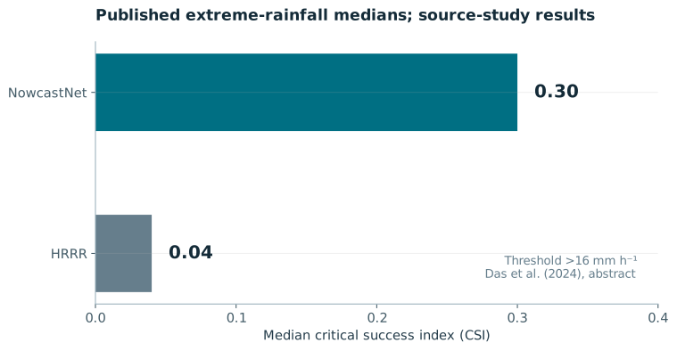
Figure 1. Published median CSI transcribed from Das et al. (2024), abstract, for grid-cell extremes above 16 mm h⁻¹: NowcastNet 0.30; HRRR 0.04. No event-level data or uncertainty intervals are reconstructed here. Download figure data (CSV).

The interpretation is stronger when event detection and water totals are read together. A forecast can correctly identify more extreme pixels yet place excessive rainfall across a basin. Hydrological utility therefore cannot be inferred from one categorical statistic. The source study motivates a multi-metric replication rather than the adoption of its headline as an expected local result.

3. Evolution constraints and what they conserve

A useful starting point for a transported image field R is an advection equation with a source term. It encodes motion and local growth or decay. The link from that image field to atmospheric mass must be stated separately. Radar reflectivity and surface rain rate are not conserved atmospheric water densities, and reflectivity in logarithmic units requires particular care.

\frac{\partial R}{\partial t} + \mathbf{u} \cdot \nabla R = S_{R}

(1)

R: rain-rate proxy or explicitly defined image field; u: horizontal motion; Sᵣ: diagnosed or learned intensity tendency.

\frac{\partial R}{\partial t} + \nabla \cdot (R\mathbf{u}) = S_{R} + R\nabla \cdot \mathbf{u}

(2)

Product-rule identity: an advective image equation is not identical to a source-free conservative continuity equation when motion is divergent.

NowcastNet combines an evolution component with conditional generation; DGMR provides a distinct generative nowcasting reference. [2] [3] These architectures should not be described as solving the full moist atmospheric system. For DLEGOS, a physical moisture budget would instead evolve explicitly defined water reservoirs, surface evaporation, condensation and precipitation sinks, with consistent units and boundary fluxes. A source term fitted without independent constraints can absorb model error, so source magnitude and closure assumptions must be reported.

4. Interactive verification of displacement error

CSI = \frac{H}{H + M + F}

(3)

H: hits; M: misses; F: false alarms. True negatives are excluded. A zero denominator is undefined, not perfect skill.

The demonstration isolates one error mechanism by shifting an otherwise similar constructed storm. It shows the double penalty of location error: observed wet cells become misses and displaced forecast cells become false alarms. The apparent loss of pixel skill does not imply that the storm structure contains no useful information. Neighbourhood verification such as the fractions skill score evaluates agreement at a declared spatial scale. [4] Neither metric removes the need to evaluate accumulation and bias.

5. Proposed Caribbean replication protocol

Select complete Jamaican rainfall events using a rule fixed independently of candidate model scores. Preserve dry and moderate-rain periods so that false alarms and event selection are not hidden. Record the observation network, quality-control flags, missing-data masks and event definitions. The principal comparison should be between models issued with the same data cutoff; delayed retrievals may serve as verification targets but cannot enter an earlier forecast input.

Compare persistence, optical-flow advection, a suitable stochastic extrapolation baseline, a data-only neural model and a physics-embedded model. Where an operational numerical forecast is available, evaluate its actual issued product rather than a retrospective analysis. Regrid all forecasts with a documented operator and harmonize accumulation windows. Satellite IMERG products supply useful precipitation estimates, but their grid support and retrieval properties differ from radar and must be included in the transfer analysis. [5]

The primary end point should be chosen before testing, for example event-averaged extreme-threshold CSI at a declared lead time and spatial scale. Secondary outputs should include FSS over several scales, mean and basin-integrated rainfall bias, false-alarm ratio, detection probability and reliability for probabilistic forecasts. Use paired event-level resampling for model differences, and publish event counts and uncertainty. Treat thresholds derived from local climatology separately from the source paper’s fixed threshold.

6. Thesis contribution and limits

The contribution is the separation of three claims: published skill in a particular source study, mathematical behaviour of a hybrid formulation and untested transfer to a Caribbean domain. The supplied results justify investigating physics-embedded nowcasting. They do not remove the need to evaluate observing-system differences, rare-event uncertainty or hydrological consequences.

A successful thesis experiment would show reproducible gains on independently held-out events while maintaining acceptable spatially aggregated rainfall and calibrated uncertainty. A negative transfer result would also be scientifically useful if it identifies whether retrieval support, event regime or the evolution constraint explains the failure. The immediate next step is an accessible, versioned event archive and a common evaluation interface. NowcastNet has not been executed or retrained within this website update.

7. Mathematical derivation and development

7.1 Deriving image motion along characteristics

Consider a differentiable image field R(x,y,t) and a path whose horizontal velocity is u = (u,v). The chain rule gives the rate of change of the image value experienced along that path. Setting that material derivative to zero assumes the feature keeps its intensity while moving. Permitting a nonzero source accounts for intensity growth or decay, but adds an unknown that must be constrained. This is an image-evolution hypothesis, not a complete atmospheric water budget.

\frac{dR(x(t),y(t),t)}{dt} = \partial _{t}R + u\partial _{x}R + v\partial _{y}R = S_{R}

(A1)

u and v have distance-per-time units consistent with x and y. S_R has image-field units per time.

For constant velocity and zero source, the exact field is the initial image evaluated at the back-traced location (x−ut,y−vt). Differentiating this expression verifies the equation directly. This characteristic solution is also a useful numerical target because it separates transport error from unknown storm growth. The Clawpack reference gives the corresponding scalar advection construction; the two-dimensional worked form here is the same chain-rule extension. [6]

R(x,y,t) = R_{0}(x - ut, y - vt)

(A2)

Exact constant-velocity translation under the stated image assumptions. It does not represent convective initiation or changing microphysics.

7.2 From optical flow to a solvable local system

One pixel gives one scalar motion equation but two velocity components. This underdetermination is the aperture problem in its elementary algebraic form. A local constant-velocity assumption permits several pixel equations to be stacked. Define row k of A as (Rₓ,k, Rᵧ,k), define bₖ = −Rₜ,k, and choose a non-negative weighting matrix W. Minimizing the weighted squared residual gives normal equations. A regularizer can stabilise a nearly singular system, but it introduces a preference that must be reported.

(A^{T}WA + \lambda I)\mathbf{u} = A^{T}W\mathbf{b}

(A3)

Derived by setting the gradient of (Au−b)ᵀW(Au−b)+λuᵀu to zero. λ≥0; λ=0 requires adequate rank.

Worked example

Use two constructed gradients A = [[1,0],[0,2]] and time derivatives Rₜ = [−3,−4]. With W = I and λ = 0, b = [3,4] and the solution is u = 3, v = 2 in grid cells per time unit. If both rows instead equal [1,0], the data say nothing about v. A unique value obtained only after regularisation is selected partly by the regulariser, not measured by those gradients.

For a learned motion field, the same identifiability issue survives in a more flexible architecture. A network can use spatial context, but source and velocity remain confounded where they produce similar intensity changes. An ablation should therefore compare fixed motion with learned source, learned motion with zero source and a joint model. Inspect whether large source terms compensate for motion errors. A visually plausible evolution is insufficient evidence of a physically identified mechanism.

7.3 A conservative transport discretisation

To demonstrate transport bookkeeping separately from image matching, let q be a conserved scalar cell average on a one-dimensional periodic interval. The finite-volume update subtracts the difference of two numerical face fluxes. For positive constant velocity a, take the upstream cell value at each right face. The numerical flux is then aQᵢ and the update has a simple two-point form. This is the first-order upwind transport example used by the executable companion. [6]

Q_{i}^{n+1} = Q_{i}^{n} - \frac{\Delta t}{\Delta x}(F_{i+1/2}^{n} - F_{i-1/2}^{n}) ; F_{i+1/2} = aQ_{i} (a>0)

(A4)

Q is an explicitly conserved scalar here. Treating surface rain-rate imagery as q would require a separate physical justification.

Q_{i}^{n+1} = (1-ν)Q_{i}^{n} + νQ_{i-1}^{n} ; ν = \frac{a\Delta t}{\Delta x}

(A5)

For a>0, 0≤ν≤1 makes the update a convex combination. Negative velocity requires the opposite upstream direction.

Multiply by Δx and sum around the periodic interval. Every outgoing face flux is the incoming flux of the next cell, so the total is unchanged in exact arithmetic. With open boundaries, retain the first and last flux rather than cancelling them. The stencil also reveals a limitation: repeated convex averaging broadens sharp features. Conservation and a positivity condition do not imply that the peak or storm position is accurate.

7.4 Mesh refinement and what the test establishes

A numerical method should be checked against a known solution as resolution increases. The companion uses exact cell averages of a smooth periodic sinusoid rather than comparing a cell average against an unrelated point value. At a fixed final time, the L1 error is the mean absolute difference of the numerical and exact cell averages. The observed order from two successively refined grids is log₂(e_h/e_h/2). For this first-order example the reported order tends towards one. The generated report, rather than a hard-coded claim, is the execution record.

p_{obs} = \frac{\operatorname{log}(e_{h}/e_{h/2})}{\operatorname{log} 2}

(A6)

A convergence diagnostic over the selected smooth solution, time and mesh sequence. It is not evidence of forecasting skill.

To extend this development towards the Caribbean task, first preserve the same array, valid-time and unit contracts across persistence, optical flow and any neural model. Add masks and boundary handling before adding an adversarial or generative objective. A stochastic generator then needs an explicit conditional distribution, random-seed handling and ensemble verification. The companion does not reproduce NowcastNet training, optical-flow training or radar nowcasting performance. It supplies a transport verification tool that the larger experiment can use.

References

AI-assisted drafting and implementation. Author and supervisory review are required before submission. The source-reported rainfall campaign, independently recounted temperature scores and constructed numerical laboratory have distinct evidence scopes.

References

- [1] Das, P. et al. (2024). Hybrid physics-AI outperforms numerical weather prediction for extreme precipitation nowcasting. npj Climate and Atmospheric Science, 7, 282.
- [2] Zhang et al. (2023). Skilful nowcasting of extreme precipitation with NowcastNet. Nature, 619, 526–532.
- [3] Ravuri et al. (2021). Skilful precipitation nowcasting using deep generative models of radar. Nature, 597, 672–677.
- [4] Roberts & Lean (2008). Scale-Selective Verification of Rainfall Accumulations from High-Resolution Forecasts of Convective Events. Monthly Weather Review, 136, 78–97.
- [5] NASA GPM. IMERG Version 07 Technical Documentation. Product documentation; consult the selected run and version for latency and support.
- [6] Clawpack Riemann Book. Scalar advection and finite-volume methods. Original software documentation.