Verification, uncertainty and reproducibility for physics-informed Caribbean forecasts

Compare a reference and an estimate. Filled isometric scientific teaching instrument. The left specimen is fixed at 0.60 constructed unit. Meeting a constraint and matching an independently known reference are distinct properties. — Constructed explanatory instrument; it is not an observed atmospheric field or a trained-model result. Geometry uses Anatomy (MIT). The paper states its evidence and limits.

Research papers · Reformatted 31 Oct 2026Executed experiments and negative results ↗Theories and hypotheses ↗

Abstract

Claims about physics-informed forecasting require evidence that separates predictive skill, numerical consistency and decision relevance. This paper specifies an evaluation framework for the DLEGOS thesis series, combining categorical rainfall verification, neighbourhood agreement, probabilistic scoring and physical budgets. An interactive threshold experiment illustrates the dependence of categorical scores on event definition. Analytical and constructed examples are separated from empirical forecasts, and source-study values are identified as literature evidence. The proposed protocol uses chronological and event-aware splits, paired comparisons, uncertainty estimation and a versioned experiment manifest. The contribution is a common standard for evaluating the preceding papers and a publication boundary: no benchmark result should be inferred from an animation, a conservation identity or a source study conducted elsewhere.

Keywords: forecast verification; CRPS; CSI; FSS; uncertainty; reproducibility; Caribbean

Thesis connection. This defines the common evidence standard for all papers, including hypothesis H3 on calibrated uncertainty. Read the hypotheses.

1. Three claims that require separate evidence

A forecasting system may be numerically consistent, predictively skilful and useful for decisions. These are related but distinct properties. A closed energy ledger verifies accounting under stated equations; a withheld-observation comparison assesses prediction; an action-specific loss evaluates utility. A thesis should identify which claim each figure and experiment can support. Displaying a realistic animated field establishes none of these claims without a defined computation and evaluation.

The attached NowcastNet comparison is a useful example of why metrics must be read together: improved extreme-rainfall detection coexists with a stated concern about spatially aggregated precipitation at longer lead times. [1] This supports a verification design with complementary measures, rather than one headline score.

2. Categorical and spatial verification

CSI = \frac{H}{H+M+F} ; POD = \frac{H}{H+M} ; FAR = \frac{F}{H+F}

(1)

Thresholded event counts. Report undefined scores when denominators are zero, and distinguish false-alarm ratio from false-alarm rate.

Threshold selection determines the event being evaluated. Fixed rain-rate thresholds, accumulation thresholds and locally estimated percentiles answer different questions. Report the sampling interval and units next to every threshold. Estimate climatological thresholds on training data or a declared independent reference period. Do not tune a threshold on test results to obtain a preferred model ranking.

FSS = 1 - \frac{\sum _{i}(p_{i} - o_{i})^{2}}{\sum _{i}p_{i}^{2} + \sum _{i}o_{i}^{2}}

(2)

pᵢ and oᵢ are forecast and observed wet-area fractions within a declared neighbourhood. The all-dry denominator is undefined.

Neighbourhood agreement evaluates spatial scale explicitly. [2] A forecast displaced by a few cells can have low pixel CSI and higher agreement over a larger neighbourhood. Report the physical neighbourhood width, grid, masks and edge handling. FSS is not a rainfall-volume score; it should be accompanied by bias and accumulation diagnostics.

3. Threshold sensitivity as an executable example

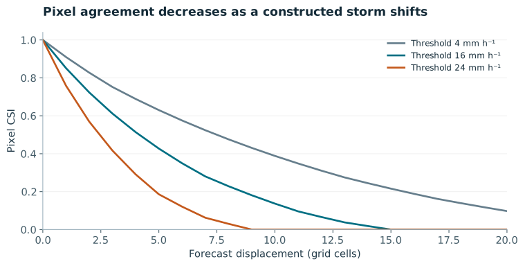
Figure 1. Computed pixel CSI against displacement for constructed Gaussian fields, at thresholds 4, 16 and 24 mm h⁻¹. Each curve is a deterministic toy calculation, not a trained-model benchmark. Download figure data (CSV).

When the threshold exceeds both field maxima, no event occurs in either mask and CSI is undefined. The interface displays this condition rather than assigning a perfect score. At lower thresholds, the storm covers more grid cells and the same displacement has a different effect. The demonstration explains metric behaviour; it cannot identify the best threshold for flood response. That choice depends on the decision and the observation support.

4. Probabilistic accuracy and physical diagnostics

\operatorname{CRPS}(F,y) = E|X - y| - \tfrac12 E|X - X′|

(3)

X and X′ are independent draws from predictive distribution F; lower CRPS is better. Units match the predicted variable.

CRPS evaluates a predictive distribution rather than a single mean. The finite-ensemble empirical-distribution form averages absolute observation differences and subtracts half the mean pairwise ensemble difference. Different finite-ensemble estimators must be labelled, particularly when ensemble sizes vary. Proper scoring rules encourage honest distributions but do not eliminate sampling uncertainty. [3]

\delta _{U}(t) = \sum _{i}U_{i}(t) - \sum _{i}U_{i}(0) - \int _{0}^{t}[S(\tau ) + B(\tau )] d\tau

(4)

Domain budget discrepancy: U is the conserved extensive quantity, S is total physical source and B is net boundary input. Analysis increments need a separate ledger.

Report budget error in physical units and with a declared normalization. A small relative residual can hide a large absolute error if the background storage is large. Separate numerical budget closure from physical model adequacy. A model can close a deliberately incomplete equation while omitting important real sources. For assimilating systems, the contribution of each observation update must be recorded instead of silently treated as physical transport.

5. Data separation, uncertainty and reproducibility

Define the independent unit before computing confidence intervals. Adjacent grid cells and consecutive radar frames are not independent weather events. Use paired event- or block-level resampling for model differences, with identical valid samples and masks. Report the number of independent events and the sensitivity to block length. A bootstrap from a small extreme-event archive is still limited by the archive; narrow pixel-level intervals do not create additional independent storms.

Freeze training, validation and test periods. Keep complete storms together, fit preprocessing only on training data and use validation data for tuning. A final retrospective retrieval can verify an earlier forecast, but a future or delayed product cannot be used as though it were available at issue time. NASA product documentation should determine the selected retrieval’s support and availability assumptions. [4] Station blending and shared analyses may reduce independence between predictors and targets and should be disclosed.

The experiment manifest should include source URLs, checksums, retrieval times, product versions, variable units, valid and issue times, masks, observation operators, splits, code commit, dependency versions, random seeds, model checkpoints and compute allocation. Save individual predictions and event-level metrics so that aggregate claims can be recalculated. Include failed runs and exclusion reasons when they affect interpretation. A random seed alone is not a reproducibility record.

6. A publication standard for the thesis series

Paper 1 establishes the conserved variable and discrete ledger. Paper 2 defines the precipitation transfer question. Paper 3 links measurements to model support. Paper 4 specifies conservative graph interfaces. Paper 5 separates foundation-model context from physical corrections. This paper supplies their shared evaluation contract. The connections should support one central scientific question rather than create several disconnected claims of novelty.

A manuscript can report an analytical result when its assumptions and derivation are explicit. It can report a literature finding when its source and evaluated domain are clear. It can report new forecasting performance only when the corresponding data, predictions and evaluation are available. The present website series contains formal methods, critical synthesis, analytical demonstrations and proposed protocols. Its next step is the common empirical benchmark; it is not yet a completed thesis or a set of peer-reviewed experimental findings.

7. Mathematical derivation and development

7.1 From thresholds to a complete contingency table

For an event threshold τ, define observed and forecast indicators Oᵢ=1[yᵢ≥τ] and Fᵢ=1[fᵢ≥τ] over the same valid sample mask. Hits count simultaneous exceedances, misses count observed-only exceedances and false alarms count forecast-only exceedances. True negatives complete the table but do not enter CSI. Every quantity depends on the chosen accumulation window, threshold and support; changing any of them defines a different verification question.

H = \sum _{i}O_{i}F_{i} ; M = \sum _{i}O_{i}(1-F_{i}) ; A = \sum _{i}(1-O_{i})F_{i}

(A1)

A denotes false alarms here to avoid confusing the count with the forecast indicator Fᵢ. The main text uses F for this count.

Worked example

Suppose five valid samples give observed events [1,1,0,0,1] and forecast events [1,0,1,0,1]. Then H=2, M=1, A=1 and one true negative remains. CSI is 2/(2+1+1)=0.5; detection probability is 2/3 and false-alarm ratio is 1/3. These are constructed counts for explaining the score, not a weather-model result.

An all-dry comparison has a zero CSI denominator and should be recorded as undefined. Decide how undefined event-level scores enter any aggregate before comparing models. Pooling all pixel counts and taking one ratio is not equivalent to averaging the ratios from individual storms. Both summaries can be useful, but they weight events differently and must be named precisely.

7.2 Deriving neighbourhood fractions and FSS

Let K_L be a declared averaging operator at neighbourhood scale L. Apply it to the binary fields to obtain p=K_LF and o=K_LO. The squared disagreement is Σ(p−o)². Expanding the square gives Σp²+Σo²−2Σpo. Substitution into the FSS definition shows that FSS is twice the overlap product divided by the sum of the two squared fraction norms. The alternative expression makes its symmetry and its all-zero degeneracy explicit.

FSS = \frac{2\sum _{i}p_{i}o_{i}}{\sum _{i}p_{i}^{2} + \sum _{i}o_{i}^{2}}

(A2)

Algebraically equivalent to the main-text form when the denominator is nonzero. The neighbourhood operator, mask and edge treatment are part of the metric.

For non-negative fractions, the inequality 2po≤p²+o² gives an upper bound of one. Zero overlap gives zero when a nonzero event fraction exists. Increasing the neighbourhood size can make displaced events look more similar, which is why the physical scale must be printed next to the score. This is a statement about thresholded spatial support, not a guarantee of accurate rainfall amounts or operational usefulness.

7.3 Empirical-distribution CRPS and its finite-ensemble distinction

Starting from the expectation form in the main text, replace F by the empirical distribution that assigns equal weight to M ensemble members. A draw from this distribution independently selects one member, so the pair expectation includes all M² ordered pairs, including zero self-distances. This produces the empirical-distribution CRPS. It evaluates the finite distribution actually issued.

\operatorname{CRPS}_{emp} = \frac{1}{M}\sum _{m}|x_{m}-y| - \frac{1}{2M^{2}}\sum _{m,n}|x_{m}-x_{n}|

(A3)

M≥1. With one member the second term is zero and this reduces to absolute error.

A different aim is to estimate the expectation score of an underlying distribution from independent ensemble draws. Excluding the diagonal pairs and normalising by M(M−1) removes the finite-sample bias in that pair-expectation estimate. This “fair” estimator needs at least two members and depends on the independent-draw interpretation. Correlated or weighted members need additional treatment; do not switch denominators without changing the description of the estimand.

\operatorname{CRPS}_{fair} = \frac{1}{M}\sum _{m}|x_{m}-y| - \frac{1}{2M(M-1)}\sum _{m\neq n}|x_{m}-x_{n}|

(A4)

Unbiased pair-expectation estimator under independent identically distributed ensemble sampling; M≥2.

Worked example

For members [1,3] and an observation of 2, the first term is 1. The ordered pair-distance sum is 4. The empirical-distribution score is 1−4/8=0.5, while the fair estimator is 1−4/4=0. The difference is a finite-ensemble estimand difference, not a change in the underlying two numbers. The companion verifies both calculations.

7.4 Paired comparisons and clustered uncertainty

For each independent event e, calculate dₑ = score_A,e−score_B,e on matched valid samples. The sign convention must be stated because lower CRPS and higher CSI represent improvement in opposite directions. To estimate uncertainty in a mean difference, resample complete events using the same indices for both models. If an event contains multiple correlated frames, keep those frames together. A block or storm-level design avoids pretending that every nearby pixel is an independent replication.

For overlapping forecast windows or persistent weather regimes, event boundaries themselves may not eliminate dependence. A sensitivity analysis should vary plausible block lengths or event definitions. Bootstrap percentiles describe the resampling scheme and available sample, not a guarantee about rare future regimes. Report the number of events, omitted undefined scores, the score aggregation rule and the full paired differences. Do not label a confidence interval from constructed data as uncertainty in a Caribbean forecast result.

7.5 Testing the evaluator before evaluating the model

Test an exact forecast, a completely displaced event, an all-dry field and a single-member ensemble. Specify every undefined case in the public metric contract.
Cross-check the two algebraic FSS expressions and the empirical CRPS implementation on hand-calculated arrays.
Verify that a shared mask removes the same samples from both forecasts. Test rate-to-depth conversions with a known interval.
Archive individual predictions, event definitions and model issue times. A published aggregate without those records is difficult to audit.

The development companion verifies hand-calculated CRPS and manufactured numerical transport. The browser functions separately cross-check CSI against the figure CSVs. These are evaluator and solver checks. They do not provide the observational sample needed for model comparison, confidence intervals or scientific acceptance. The companion’s report and data are available from the development laboratory, alongside the exact executable source.

References

AI-assisted drafting and implementation. Author and supervisory review are required before submission. The source-reported rainfall campaign, independently recounted temperature scores and constructed numerical laboratory have distinct evidence scopes.

References

- [1] Das, P. et al. (2024). Hybrid physics-AI outperforms numerical weather prediction for extreme precipitation nowcasting. npj Climate and Atmospheric Science, 7, 282.
- [2] Roberts & Lean (2008). Scale-Selective Verification of Rainfall Accumulations from High-Resolution Forecasts of Convective Events. Monthly Weather Review, 136, 78–97.
- [3] Gneiting & Raftery (2007). Strictly Proper Scoring Rules, Prediction, and Estimation. Journal of the American Statistical Association, 102, 359–378.
- [4] NASA GPM. IMERG Version 07 Technical Documentation. Product documentation; consult the selected run and version for latency and support.