Conservation-constrained learning for local atmospheric prediction in Jamaica

Account for one shared transfer. Filled isometric scientific teaching instrument. Two chambers begin with a combined amount of one constructed unit. The total stays fixed even if the chosen transfer is physically wrong. — Constructed explanatory instrument; it is not an observed atmospheric field or a trained-model result. Geometry uses Anatomy (MIT). The paper states its evidence and limits.

Research papers · Reformatted 31 Oct 2026Executed experiments and negative results ↗Theories and hypotheses ↗

Abstract

This paper formulates a conservation-first basis for local atmospheric learning in the DLEGOS research programme. A control-volume representation separates resolved transport, external forcing and unresolved processes. The principal argument is that physical accountability requires an auditable discrete budget, rather than the presence of a differential equation in a training objective. A reduced sensible-heat implementation provides an executable example over two Jamaican terrain domains. Its historical inputs and numerical states are explicitly distinguished from independent observations. We derive the cancellation of internal exchanges, identify the conditions under which that result holds, and define falsifiable tests for a subsequent learned model. No new forecast-skill claim is made: the contribution is a formal specification, a traceable numerical demonstration and a validation design.

Keywords: conservation; finite volumes; physics-informed learning; Jamaica; atmospheric modelling

Thesis connection. This establishes the reduced conservation ledger used by the coupled model. The space–time formulation is defined in Paper 0. Read the hypotheses.

1. Scientific question and scope

The central question is whether explicit conservation constraints improve local atmospheric prediction when observational coverage is limited and the prediction grid is finer than the available meteorological inputs. This question requires separate assessments of predictive accuracy and physical consistency. A field may fit observations while accumulating an unphysical energy surplus; a conservative field may still place rainfall incorrectly. The thesis should therefore treat conservation as a testable property and possible source of inductive bias, rather than as sufficient evidence of forecasting skill.

DLEGOS represents a spatial cell together with its time history. The term “tesseract” names that computational object; it does not assert that the atmosphere requires a fourth spatial dimension. The current website integrates a reduced temperature model above real terrain. Momentum, water species, clouds and precipitation remain extensions to the research architecture. The formal atmospheric reference is the WRF technical formulation, which must be adapted with explicit approximations rather than copied as a list of disconnected equations. [1]

2. Control volumes and the discrete energy budget

Let cell i have fixed volume Vᵢ, constant reference density ρ and heat capacity cₚ. Under this reduced model, Eᵢ = CᵢTᵢ, where Cᵢ = ρcₚVᵢ. This quantity is a sensible-heat storage variable under prescribed material properties; it is not total moist atmospheric energy. Neglecting kinetic, latent and gravitational energy is a substantive approximation. For each shared face, choose one exchange Qᵢⱼ and apply its negative to the neighbouring cell.

E_{i}^{n+1} = E_{i}^{n} + \Delta t [ \sum _{j\in N(i)} G_{ij}(T_{j}^{n} - T_{i}^{n}) + S_{i}^{n} ]

(1)

E: sensible-heat storage (J); G: symmetric face conductance (W K⁻¹); S: prescribed heating (W); Δt: step length (s). This is the reduced model, not a complete atmospheric energy equation.

Summing over cells pairs each internal face contribution with its negative. The proof needs symmetry of Gᵢⱼ, a shared numerical evaluation of the face flux, consistent time integration and explicit accounting for boundary contributions. If two networks independently predict the two sides of a face, cancellation is no longer guaranteed. A single learned face flux, assigned with opposite signs, provides a stronger structural constraint.

\sum _{i}(E_{i}^{n+1} - E_{i}^{n}) = \Delta t \sum _{i}S_{i}^{n}

(2)

Closed outer boundary: internal transfers cancel exactly in algebra. Floating-point accumulation introduces a small numerical remainder.

The implemented conductance is ρcₚκAᵢⱼ/dᵢⱼ, with prescribed diffusivity κ, shared area A and centre separation d. The explicit update must respect a stability limit determined by each cell capacity and the sum of its conductances. Small terrain-cut cells deserve particular attention because their storage capacity can be small relative to the exchanging face area. The six-hour relaxation and illustrative solar heating in the existing workbench are external terms in the ledger; neither is an internal conservative exchange.

3. From a physical residual to a learning objective

Physics-informed neural networks constrain fitted functions with differential residuals. [2] For this application, the proposed learning objective should also include a discrete budget residual evaluated using the same operators as the numerical update. Otherwise, a small continuous residual at selected collocation points may coexist with a biased integrated budget. All residuals should be nondimensionalized before their weights are interpreted.

\mathcal L(\theta ) = \mathcal L_{obs} + \lambda _{r}\mathcal L_{res} + \lambda _{b}\mathcal L_{boundary} + \lambda _{c}\mathcal L_{budget}

(3)

θ: trainable parameters. Each loss is normalized by a declared scale; λ terms are selected using validation data only.

Two alternatives warrant comparison. A soft-constraint model penalizes budget error but can violate it. A structural model predicts shared face exchanges and permitted source terms so that internal cancellation follows by construction. These alternatives answer different questions. Demonstrating exact cancellation in the structural model confirms its implementation, while demonstrating improved independent predictive skill would require withheld observational evaluation. Neither should be reported as the other.

4. Executable demonstration and historical context

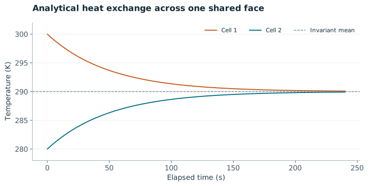
For two equal capacities, the mean temperature is invariant and the difference decays as exp(−2kt). The interactive figure computes this exact solution; it does not train a network or solve the full atmosphere. Increasing coupling accelerates equilibration without creating heat. The corresponding static chart permits direct inspection of the time scale.

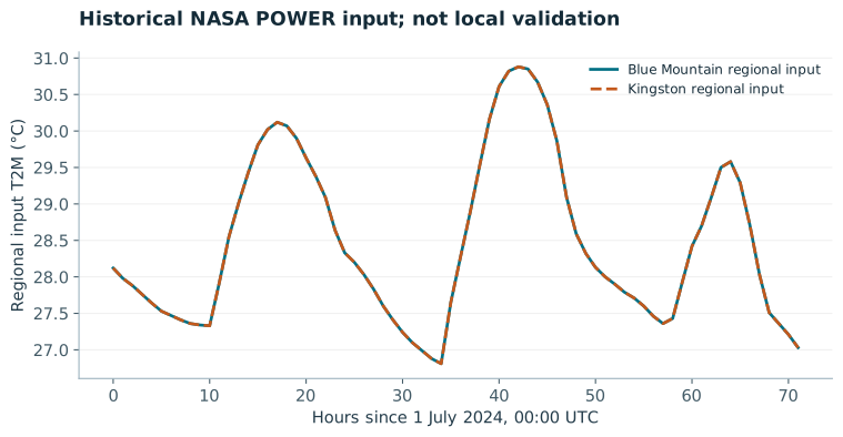
Figure 1. Exact two-cell exchange: T₁(0)=300 K, T₂(0)=280 K and G/C=0.01 s⁻¹. The arithmetic mean remains 290 K. Download figure data (CSV).

Figure 2. Existing NASA POWER regional T2M inputs for the Blue Mountain and Kingston domains, 1–3 July 2024 UTC. Identical or similar curves reflect coarse source support, not independent local thermometers. Download figure data (CSV).

The historical curves are reproduced from source responses already stored with the workbench. [3] They are contextual input data, not a validation sample. Their coarse spatial support cannot establish that a one-kilometre model resolves local terrain-driven circulation. The numerical replay can be audited against its input and energy ledger, but an accuracy assessment requires independent station or field measurements.

5. Experimental design and falsification criteria

The proposed comparison holds architecture capacity, input variables, training dates and optimization budget as constant as practicable while changing the constraint mechanism. Evaluate an unconstrained network, a residual-penalty network and a shared-flux model against a persistence baseline and the same reduced numerical model without learning. Use chronological splits with entire weather events excluded from training and tuning. Where stations permit, withhold complete locations to distinguish interpolation from transfer.

Report temperature error by lead time, elevation band and weather regime alongside normalized budget drift. The primary hypothesis is that a conservation constraint reduces drift without degrading independent predictive accuracy beyond a prespecified tolerance. A model that conserves energy but performs worse than persistence does not support a useful prediction claim. If the apparent improvement disappears when boundary forcing and assimilated observations are held equal, the improvement should be attributed to information access rather than to the constraint.

6. Interpretation, limitations and thesis contribution

The formal result is conditional but exact: pairwise antisymmetric internal exchanges cancel in the domain sum. The empirical question remains open. In particular, constant density, prescribed diffusivity and a temperature-only storage variable exclude important atmospheric mechanisms. Radiative forcing, surface exchange and analysis increments require separate accounting. Extending the same ledger to moisture and momentum will require a consistent thermodynamic state and selected closures, not merely additional loss terms.

This paper supports the thesis by fixing the physical object being learned and the standard of evidence required to assess it. Its immediate next step is an independent observational benchmark with frozen operators, archived parameters and a conservation ablation. The website implementation demonstrates bookkeeping and mathematical behaviour; it does not establish a new Jamaican forecasting capability.

7. Mathematical derivation and development

7.1 From a local balance to an extensive cell update

The reduced thermal model can be derived without starting from a neural network. Take a fixed control volume Ωᵢ and define its storage as the integral of ρcₚT over that volume. Here ρ and cₚ are prescribed reference properties, the geometry is fixed, and the reduced model represents sensible heat only. Let F denote an outward energy flux density, in W m⁻², and let s denote volumetric heating, in W m⁻³. Applying the divergence theorem converts a volume divergence into face integrals. The sign convention matters: a positive outward face flux removes energy from the cell.

E_{i} = \int _{\Omega _{i}}\rho c_{p}T dV ; \frac{dE_{i}}{dt} = -\oint _{\partial \Omega _{i}}\mathbf{F} \cdot \mathbf{n} dA + \int _{\Omega _{i}}s dV

(A1)

Ωᵢ: fixed cell; n: outward normal; Eᵢ: reduced sensible-heat storage in J. This derivation assumes constant reference density and heat capacity.

For a well-mixed cell, pull Tᵢ outside the storage integral and define Cᵢ = ρcₚVᵢ. Approximate the conductive or diffusive flux using the difference between neighbouring cell temperatures and one shared interface conductance. A larger shared area increases transfer; a larger centre separation reduces it. The diffusivity κ is a model parameter in this reduced system. It must not be confused with resolved wind advection or molecular thermal conductivity.

G_{ij} = \rho c_{p}\kappa \frac{A_{ij}}{d_{ij}} ; C_{i}\frac{dT_{i}}{dt} = \sum _{j}G_{ij}(T_{j} - T_{i}) + S_{i}

(A2)

Cᵢ: J K⁻¹; Gᵢⱼ: W K⁻¹; Sᵢ: W. The units on both sides of the temperature equation are W.

This is a derived finite-dimensional model, not a claim that all terms of atmospheric thermodynamics have been retained. A moist compressible extension would require compatible mass, momentum, thermodynamic and water-species variables, with pressure work, latent processes and boundary exchange treated consistently. The atmospheric equation families and coordinate choices are documented in the WRF technical note cited in the main text. The present derivation intentionally stops before those unresolved closure choices.

7.2 Deriving a stable explicit time step

Forward Euler replaces the time derivative with a finite difference evaluated at the old state. Divide by Cᵢ and collect the coefficient multiplying Tᵢ. With no external forcing, the update is a convex combination of old temperatures when every coefficient is non-negative and their sum is one. This yields a sufficient maximum-principle condition, stronger in meaning than simply observing that a short animation looks stable.

T_{i}^{n+1} = (1 - \Delta t \sum _{j}G_{ij}/C_{i})T_{i}^{n} + \sum _{j}(\Delta t G_{ij}/C_{i})T_{j}^{n}

(A3)

Derived by expanding equation (A2); all conductances are non-negative and are frozen during this step.

0 \leq \Delta t \leq \operatorname{min}_{i:\sum G_{ij}>0} \frac{C_{i}}{\sum _{j}G_{ij}}

(A4)

Sufficient convexity bound for pure diffusive exchange. Isolated cells impose no diffusion bound. External relaxation and other explicit terms can tighten the condition.

Worked example

Let C₁ = 2 J K⁻¹, C₂ = 1 J K⁻¹, G₁₂ = 0.1 W K⁻¹ and Δt = 1 s. Starting from 300 K and 280 K, the transfer is 2 J from cell 1 to cell 2. The temperatures become 299 K and 282 K. Initial energy is 880 J and final energy is 880 J. Equal temperature changes of −2 K and +2 K would instead give 878 J, because the capacities differ. These deliberately small capacities are constructed numerical values, not atmospheric cell capacities.

If a six-hour temperature relaxation is added, its coefficient contributes 1/τ to the diagonal decay rate. The non-negative self-weight then requires Δt(ΣGᵢⱼ/Cᵢ + 1/τ) ≤ 1 for this combined Euler update. A prescribed source independent of T changes the budget but not that linear coefficient. Clipping a negative or overshooting state after a step generally adds an unrecorded correction; if clipping is used, it needs its own ledger and cannot be described as an automatically conservative repair.

7.3 Nondimensional physics residuals and loss gradients

Let x = Lx̃, t = τt̃ and T = T₀ + ΔT T̃. The diffusion term then introduces the dimensionless group κτ/L². A residual evaluated in K s⁻¹ cannot be added meaningfully to an observation error evaluated in K² without a declared scaling. One practical construction first scales each residual by a physically chosen tendency scale ΔT/τ, and each observation error by ΔT. The numerical values of loss weights then have an interpretable reference.

r = \frac{\tau }{\Delta T} [\partial _{t}T - \kappa \nabla ^{2}T - s_{T}] ; \mathcal L_{res} = \frac{1}{N_{r}} \sum _{k}r_{k}^{2}

(A5)

s_T is a temperature tendency in K s⁻¹. L, τ and ΔT must be fixed from physical design or training data, never selected using test outcomes.

When T is represented by a differentiable network, the physics loss depends on derivatives of its output as well as on the output itself. Differentiating that loss with respect to network parameters therefore requires the derivative computation to remain part of the parameter graph. The NumPy companion takes a different, explicit route: it learns face conductances and derives the parameter gradient of a discrete tendency loss by the chain rule. Paper 4 gives that derivation. The two approaches are related by their use of physical operators, but they are not interchangeable implementations of the same PINN.

7.4 Development sequence and stopping conditions

Implement storage, shared faces and boundary fluxes independently of learning. Verify signs with a two-cell calculation before building a large grid.
Validate the explicit step against the capacity-dependent bound. Test a closed domain, a forced domain and deliberately inconsistent opposite-face values.
Add one unknown parameter or closure, not all atmospheric physics at once. The companion learns positive conductances on a constructed closed graph.
Separate state error, source error and budget error. Publish each separately; a small budget remainder does not establish that the physical approximation is adequate.

The companion makes these checks executable with step, rates, graph_system and the closed-rollout ledger. Its small neural model is a development test. The current Jamaican terrain replay remains a reduced prescribed-forcing model; neither the new tests nor the animation establish a trained atmospheric PINN.

References

AI-assisted drafting and implementation. Author and supervisory review are required before submission. The source-reported rainfall campaign, independently recounted temperature scores and constructed numerical laboratory have distinct evidence scopes.

References

- [1] Skamarock et al. (2019). A Description of the Advanced Research WRF Model Version 4. NCAR Technical Note NCAR/TN-556+STR.
- [2] Raissi, Perdikaris & Karniadakis (2019). Physics-informed neural networks: A deep learning framework for solving forward and inverse problems involving nonlinear partial differential equations. Journal of Computational Physics, 378, 686–707.
- [3] NASA POWER. Hourly point API: historical source response embedded in the DLEGOS workbench.