Keywords: atmospheric reconstruction; finite volumes; conservative coupling; incidence matrix; identifiability; data assimilation; moisture transport; Jamaica.
1 Introduction
The organising task is retrospective reconstruction of rainfall-relevant atmospheric structure over Jamaica and, later, other Caribbean islands, under sparse observations and a large-scale background that may be biased. The question is conditional. Under which combinations of observation coverage, driver error and interface formulation does physical coupling between local models improve the recovered moisture transport, and under which does it transmit the driver’s error? Weather prediction, climate response and impact modelling are separate extensions with separate evidence requirements.
The nearest lineages are finite-basis and domain-decomposed physics-informed networks [1, 2], conservative PINNs [3], hard-constrained downscaling [4], probabilistic conservation [5] and weak-constraint variational assimilation [6]. Exact algebraic cancellation is not claimed as new, and the use of local networks is a representation choice without any standing as a physical principle. This paper defines the learned state, its required numerical ledger, the limits of that ledger and the evidence needed to establish an improvement. The component studies that have been run so far (rainfall allocation, temperature correction, a synthetic closure experiment and a soil-temperature operator study) are cited where they bear on the design; none of them is the atmospheric reconstruction.
2 Space-time control volumes
Let be a spatial control volume and a time interval; the computational block is with normalised coordinates . When is a cube the block has the topology of a four-dimensional hypercube: 16 vertices, 32 edges, 24 square faces and eight cubic facets, of which two are the spatial volume at the start and end of the interval and six are the spatial faces swept through time. The scales and are prescribed. Drawings are projections of the space-time block; time retains its stated units.
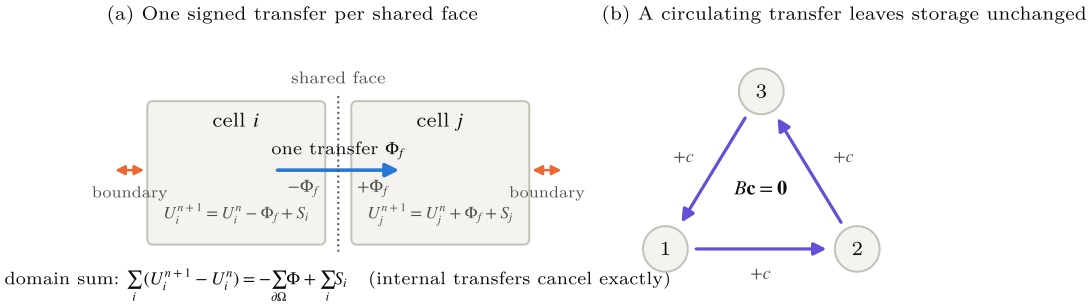
For an extensive density , flux and source with , integrating over and then over gives (1) With the cell integral, the integrated outward transfer through face and the integrated source, a shared face between and has when one transfer is assigned with opposite orientations, and (2) Fixed geometry is assumed; moving boundaries need the relative flux and terrain-cut volumes need correct measures. For total atmospheric water the state must include the chosen water species and every transfer the closure represents; a vapour equation alone supplies no microphysics, and a vertically integrated budget needs explicit conventions for condensate storage, the model top and the lower boundary, with any analysis increment booked in the source ledger. Moisture budgets computed from analysed products are sensitive to discretisation [7], which is why the baseline residual of the background itself is measured before any reconstruction is credited.
3 A reduced sensible-heat system
A reduced sensible-heat system illustrates the accounting before atmospheric reconstruction is attempted. Let cell have fixed volume , reference density and heat capacity , storage with , and one exchange per shared face. The explicit update is (3) with for prescribed diffusivity , shared area and centre separation . The proof of the second equality needs symmetry of , one shared numerical evaluation of the face flux, consistent time integration and explicit boundary accounting; if two networks predict the two sides of a face independently, exact cancellation generally fails. A worked example makes the capacity point: with , J K, W K, s and temperatures 300 and 280 K, the transfer is 2 J, the temperatures become 299 and 282 K and the energy stays at 880 J, whereas equal-and-opposite increments of 2 K would give 878 J.
Dividing by and collecting the coefficient of writes the unforced update as a convex combination of old temperatures whenever (4) a sufficient maximum-principle bound; a relaxation term with time scale tightens it to . Small terrain-cut cells with large faces are where this binds. Clipping an overshooting state adds an unrecorded correction and needs its own ledger. Non-dimensionalising with , , introduces the group , and a residual in K s is scaled by before it is added to an observation error scaled by ; loss weights then have a reference. The learning objective pairs the usual observation, residual and boundary terms with a discrete budget residual evaluated by the same operators as the numerical update, because a small continuous residual at collocation points can coexist with a biased integrated budget. A soft budget penalty and a structural shared-flux model answer different questions. Exact cancellation in the structural model confirms its implementation; improved withheld skill needs observational evaluation; neither should be reported as the other.
4 Oriented graphs, incidence and a learned positive closure
4.1 Incidence form
Orient each internal face once and let have at the receiving cell and at the sending cell. For an extensive stored vector , edge transfer rates and external sources , (5) A neural edge function may produce from neighbouring states, geometry and context; using the same at both endpoints preserves cancellation and guarantees nothing about stability, positivity, constitutive accuracy or boundary forcing. For unequal capacities a transfer changes temperatures by and . With the receiver-minus-sender difference and for positive conductances, (6) so the constant vector is in the null space of and a uniform temperature has zero tendency, a second implementation check beyond total closure, since a sign error can preserve a sum while moving heat between equal cells.
Proposition 1 (Dissipation, separate from conservation). Let and . For ,
Proof. is invariant because ; differentiate and substitute; the constant component vanishes under . ◻
Total reduced energy is constant while temperature differences dissipate; is a variance-like functional, not an entropy. Non-negative does not make large Euler steps stable, a state-dependent learned must be evaluated at the old state and the bound of Equation 4 rechecked, and a positive diffusive closure may be the wrong class for advective or counter-gradient processes however easy it is to stabilise.
4.2 Executed closure test
The executable companion fits an edge multilayer perceptron (three dimensionless edge descriptors, one tanh layer of eight units, scalar output through softplus with W K and ) to constructed temperature tendencies on a closed 12-cell chain with 11 edges, using a hand-derived backward pass checked against centred finite differences and Adam. The recorded run (seed 23, 1,200 iterations, 192 training and 96 held-out fields on the same graph) reaches a final training tendency MSE of K s and a held-out tendency RMSE of 0.00346 K s−1, against 0.634 for an untuned fixed conductance W K; the learned conductances have RMSE W K against the generating values. The largest relative gradient discrepancy is ; the convexity bound is 1.37 s and the rollout step 1.09 s; the maximum closed-rollout energy drift is J while the weighted variance falls from 48.4 to 0.0011 J K. A companion upwind advection ladder over 32 to 256 cells at Courant 0.597 has zero mass drift and observed orders of 0.977, 0.988 and 0.994. Every training target comes from the declared diffusion operator, so this is a manufactured inverse-model development exercise; it tests the bookkeeping and the gradient, not the atmosphere, and the untuned comparator must be replaced by a fitted constant before any learned-closure advantage is claimed. [from development/results/report.json]
5 The restricted atmospheric class and its parameterisation
The first real-atmosphere inference uses hydrostatic mesoscale fields on pressure surfaces at the scale resolved by an ERA5 background [8]: horizontal wind , temperature and specific humidity as unknowns; geopotential diagnosed hydrostatically from virtual temperature with a boundary value; pressure velocity taken from the background in the first comparison and later diagnosed from continuity, never a free network output; surface pressure, terrain masks and lateral background retained with their uncertainty, and terrain-intersecting levels masked rather than interpolated. The resolved balances, in the form documented for the IFS [9] but reduced to pressure coordinates, are (7) with and . Hourly sampling does not resolve hourly convection and a fine output grid does not change the approximation; kilometre-scale convective cells are outside the claim. The unresolved tendencies , and are the most important restriction. They are prescribed from a documented reference or bounded by a stated prior, never free functions tuned until every residual vanishes, so a wrong closure appears as reconstruction error instead of being absorbed. Joint state-and-closure learning is a different inverse problem and is deferred.
A local neural field maps normalised coordinates and admissible context to the resolved variables; a partition of unity blends overlapping fields, and smooth blending alone does not make fluxes conservative, so the shared transfer is defined separately on the faces. A reference architecture is a two-layer, 64-unit tanh trunk with outputs after variable-specific scaling and softplus-bounded humidity; derivatives keep their dependence on the parameters, since computing a residual and detaching it would remove the physics gradient. The objective is (8) with the observation operator at the measurement’s own support, the non-dimensionalised residual of the balances above, the interface term that defines the coupling variant and the boundary term. Under Gaussian assumptions this is the weak-constraint 4D-Var objective [6] with the model-error term evaluated as a residual on the continuous field rather than a discrete forecast step; the field changes the parameterisation and removes neither the inverse problem nor the identifiability question. Covariances carry the evidential weight. comes from the ERA5 ensemble spread with localisation and inflation if the simulation shows over-confidence; from instrument specifications plus a representation term from station-background mismatch over a training period; tuned where truth is known and then frozen. If covariances are estimated jointly with the state, the log-determinant terms must be kept, otherwise the optimiser is rewarded for inflating a covariance against a non-zero residual.
Filtering, smoothing and forecasting differ in the evidence they may use, which is , with , and respectively; the direction in which a network is evaluated has nothing to do with it. The primary task is smoothing, which may use observations from before, during and after an event and whose scores cannot be compared with a forecast issued before the later observations existed. Dissipation is the concrete obstacle to anything resembling time reversal. A Fourier mode of the heat equation decays as and backward inversion amplifies the smallest-scale noise by the reciprocal, so a visually reversible display re-indexes stored observations and does not solve a stable inverse equation.
6 What conservation does not prove
The algebra above is exact under its assumptions. The same algebra bounds what it can be used to claim. The statements below are elementary; each was recomputed numerically for this draft (Section 9).
Proposition 2 (Samplewise ledger). With one transfer per internal face used with opposite signs, internal transfers contribute nothing to the domain-total tendency for every ensemble member, not only in expectation: for , for any .
The identity says nothing about the accuracy of the sample or of the external terms, and it holds for the discrete update only if one time-integrated transfer is used on both sides of each face; separate quadrature of the two sides breaks it.
Proposition 3 (Local uncertainty depends on cross-face covariance). For an ensemble conditioned on the same assimilated observations with fixed external terms, . For a column with faces 12 and 23, .
Independent face samples therefore keep the ledger exact and mis-state local uncertainty by an amount set by the omitted covariance; positive covariance makes independence too wide, negative too narrow. A shared low-rank representation with an orthonormal basis [10] gives and can represent dependence; it does not guarantee the right dependence, and rank, basis and reference law are chosen on development data only. Stochastic separable PINNs [11] are a candidate representation for the coefficients; calibration of the resulting posterior is a separate test.
Proposition 4 (Cycle ambiguity). If observations constrain only the storage trajectory and the external terms, any flux perturbation with leaves the trajectory unchanged, and on any graph with a cycle such non-zero exist.
A circulating transfer around a closed loop enters and leaves each participating column equally. Storage-only likelihoods cannot distinguish it; a prior can select a member of the equivalence class without converting that selection into identification; independent wind or humidity-profile information is what constrains it. On the 12-cell chain of the executed test the cycle space is empty, which is one reason that test cannot exhibit the ambiguity.
Proposition 5 (False precision from a biased background). With truth , observation , , and a fixed Gaussian prior with mean and variance , the posterior mean is with and reported variance , while and .
As the reported variance tends to zero and the bias to . This motivates the bias stress tests in the protocol; it estimates no atmospheric bias and does not say that wider intervals improve a proper score.
Proposition 6 (Constraint compatibility at the represented scale). Let aggregate a fine state, and be the corresponding linear constraint operators and a bounded map between their outputs. With the defect , a fine state with has coarse residual , and in general .
A non-zero coarse residual can arise from incompatibility alone. The result of [12] that only linear constraints survive coarse-graining assumes translation-invariant filtering and constant coefficients on a periodic domain; pressure coordinates, spherical geometry, terrain masks and a moving surface pressure require the defect to be computed, not assumed away. For a plain average the unresolved product has velocity units and is not yet a transport; it needs pressure, area and time weights before it can enter the ledger. The incidence identity is independent of this defect and cannot establish that a transfer represents resolved transport or that the unresolved term is negligible. Before inference, the state variables, aggregation and constraint operators, units, boundary conventions, masks and tolerances are frozen, and is computed on constant-field, boundary and terrain cases at native and reconstruction support.
7 Hypotheses, variants, baselines and protocol
7.1 Coupling variants and baselines
For block with faces , orientation and face measure , the integrated vapour budget is , and the variants differ only in how is obtained at a shared face. C0 is uncoupled, with no interface term. C1 is state-matched: a penalty on differences of at shared faces, so the fluxes implied by each side may still differ. C2 is penalised flux: a penalty on , which encourages continuity. C3 is shared signed flux: one computed from both fields, entering with and with , so internal transfers cancel exactly. C3 guarantees an accounting identity only; accuracy, humidity positivity and numerical stability are separate measured questions. Baselines are B0 the background without adjustment, B1 a seasonally and terrain-conditioned regression or optimal-interpolation statistical reconstruction, B2 a single non-decomposed field with the same total capacity, and B3 an ensemble Kalman smoother or weak-constraint 4D-Var with the same window. Parameters, observations, epochs and tuning budget are matched between B2 and C0 to C3 and reported for all; a mechanism comparison holds them fixed and a best-configuration comparison is reported separately and labelled.
7.2 Domain, stages and events
The proposed domain is 14–22N, 82–72W, about cells at 0.25, large enough to capture inflow along the Caribbean low-level jet and to be tested against a smaller and a larger domain first, following the domain-size sensitivity found in regional modelling [13]; pressure levels from 1000 to 200 hPa with terrain masking; block sizes of 1, 2 and 4 with and without one-cell overlap, with the number of observations per block reported and sizes that leave most land blocks unobserved flagged; a window of about 72 h around the event peak. Stage 1 is an observing-system simulation experiment [14] whose nature run comes from a different system than the background to avoid the identical-twin problem; it varies observation density, removes vertical information and perturbs prescribed tendencies, tunes and sets minimum detectable effects. Stage 2 uses observed events across five regimes (tropical cyclone, early-season rainfall, mid-summer minimum, late-season non-cyclone rainfall, dry spell) with withheld stations, any radiosonde ascents, gauges not in the reference product and independently computed budget terms; an unobserved transport field is never described as validated because it agrees with the background.
7.3 Three hypotheses and their pre-analysis plans
Observation masks, sparsity levels, bias levels and metrics are fixed before any Stage 2 evaluation; selection, calibration and testing use separate events; calibration is frozen before final scores; intervals on paired differences use a block bootstrap with events as the unit [15].
H1 (exact aggregation under driver bias). Under accurate coarse forcing, exact aggregation preserves or improves independently evaluated precipitation allocation relative to a matched unconstrained learner; as driver bias grows the advantage shrinks and may reverse. The manipulated factor is multiplicative bias at 0, , , % plus spatial displacement; the outcome is error at withheld gauges not used by the reference; support requires constrained error at or below unconstrained at zero bias and a paired difference that grows with bias, with the crossover estimated rather than assumed. The executed CHIRPS component study already shows the mechanism in its conditional form. Exact conservation helps a matched network, loses to a climatological allocation, and transmits a % driver error into an aggregation floor of 31.67 mm/month.
H2 (flux coupling under sparse observations), the principal experiment. With matched observations, capacity and compute, C3 gives lower withheld moisture-transport error than C1, C2, C0 and B2, and the advantage grows as coverage falls. The manipulated factor is the fraction of the network retained (100, 50, 25, 10 %) and vertical data on or off; the outcome is vector error in and in moisture-flux convergence against the nature run, and withheld and wind in real events; support requires the C3 minus C1 paired difference to be negative with a 95 % interval excluding zero at the two sparsest densities and not to favour C1 at full density by more than the minimum detectable effect. Exact interface agreement can coexist with rejection of H2 if wrong closures or boundaries worsen interior recovery.
H3 (uncertainty from background and model discrepancy). Representing background and discrepancy uncertainty explicitly improves probabilistic reconstruction relative to a matched model that treats them as fixed. Wider intervals alone do not support it. The outcome is CRPS for withheld quantities, coverage of 90 % intervals within a prespecified band without interval width growing beyond a stated limit, and energy and variogram scores for joint structure [16, 17]. A nested sub-analysis compares shared-latent and face-local latent inference families through the same state-flux-compatible map, with the energy score of a fixed vector of column moisture tendencies as the primary score and a pilot-defined negative benefit margin that the upper endpoint of the paired interval must clear. A deterministic fit with a separately calibrated residual distribution remains a baseline.
7.4 Verification and reporting
Splits are by whole event or contiguous time block; leave-island-out is reserved for any transfer claim; random pixel withholding is not used. Continuous error (RMSE, bias) by pressure level, land or sea and terrain class; threshold and spatial skill (CSI, Brier, fractions skill score at stated neighbourhoods [18]); probabilistic scores; and physical diagnostics (signed and absolute budget residuals per block and domain against the background’s own residual, computed with an independent discretisation at locations not used in fitting) are reported separately, with no combined score. Key results are repeated against an alternative rainfall reference. The threats to validity and their mitigations are fixed in advance (Table 1). A retrospective smoother has no licence to favour a desirable outcome, so no planning or optimism term of the kind used in test-time world-model adaptation [19] enters the objective.
Three outcomes count as results, and each answers the research question: coupling helps in a stated regime; coupling transmits a biased background; the observations cannot distinguish competing states.
| Threat | Mitigation |
|---|---|
| Gauge overlap between training and verification | Audit; verify only on non-contributing gauges |
| Identical-twin optimism | Nature run from a different system than the background |
| Gains from tuning or capacity | Matched budgets; compute reported |
| Wrong prescribed tendencies | Perturbed-tendency sensitivity, reported as reconstruction error |
| Interface diagnostics that repeat the objective | Independent discretisation on held-out faces and times |
| Masks tuned to outcomes | Frozen before Stage 2 |
| Too few events | Power analysis from Stage 1 |
| Reference-product dependence | Repeat with a second product |
The design cannot show convection-permitting skill, operational forecast skill or anything about future climate statistics, and hybrid models validated as global forecasters [20] and forecasting benchmarks [21] are precedents for evaluation conventions, not evidence for this smoother.
8 Evidence from the component studies
Four executed component studies inform the proposed atmospheric protocol. The rainfall allocation benchmark shows an exact volume constraint improving a matched network and losing to a seasonal climatological allocation, with the aggregation floor making the H1 mechanism concrete. The temperature study shows a reduced relaxation-radiation-ocean closure giving a conditional gain inside a symmetric exchange graph while a frozen foundation model remains the stronger reference, which is a caution for H2 about what a symmetric, distance-based exchange can represent. The synthetic closure experiment shows a learned source compensating a wrong wind while the ledger stays at machine precision, which illustrates transport-source ambiguity, and an adaptive tolerance failing to beat ordinary pooling. The soil-temperature operator study shows a satisfied pointwise operator budget coexisting with no reconstruction gain, which is the distinction between the ledger and accuracy that this paper makes formally. None of them is the atmospheric reconstruction and none changes the hypotheses; together they are the reason the hypotheses are stated with the decision rules above rather than as expectations.
9 Numerical checks of the propositions
A short script accompanying this draft recomputes each analytic statement with independent code. The two-cell worked example gives 2 J transferred, 880 J before and after, and 878 J under equal increments. With the capacities reversed (, J K at the same temperatures) the common equilibrium is 286.67 K, where equal capacities would give 290 K. For the 12-cell chain, , the rank is 11 and the cycle space is empty; for a 3-cycle, is a non-zero null vector with to machine precision. The cross-face variance identity holds on 200,000 correlated draws: 0.802 empirical against 0.8 from the formula with , where independence would give 2.0. The biased-background bias and mean-squared error on 400,000 draws are 1.334 and 1.890 against 1.333 and 1.889 from the formulae. On a random 12-chain the convexity bound produces no new extrema inside it with energy drift of , the dissipation rate is negative, and the compatibility defect is non-zero for a varying velocity and exactly zero for a constant one. These checks test the algebra. Atmospheric performance remains to be evaluated under the proposed protocol. [from the accompanying analytic-check script]
10 Limitations
The formal results are properties of stated graphs and scalar models. They do not prove non-negativity of humidity, stable atmospheric integration, identifiable fluxes or calibrated uncertainty; those are the measured questions in the protocol. Hydrostatic reconstruction at the background’s resolved scale is not convection-permitting simulation. Geometry, representation error, conditional-sampling quality and model discrepancy may dominate any uncertainty representation. The executed closure test is on a constructed chain with no cycles, no noise, no missing observations and no unseen geometry. The nearest existing methods already contain conservative updates, discrepancy learning and probabilistic conservation, so any additional contribution depends on the integrated formulation and the evidence from its proposed evaluation; the identities are established results. The next step is Stage 1, run so that H2 can be rejected.
Data and code availability
The analytic-check script and the 12-cell closure test (code, seed, training and held-out fields and the results report) are held in the programme repository and are available on request. No atmospheric data were used in this paper.
References
[1] Ben Moseley, Andrew Markham, and Tarje Nissen-Meyer. Finite basis physics-informed neural networks (FBPINNs): a scalable domain decomposition approach for solving differential equations. Advances in Computational Mathematics, 49: 62, 2023. doi: 10.1007/s10444-023-10065-9.
[2] Ameya D. Jagtap and George Em Karniadakis. Extended physics-informed neural networks (XPINNs): A generalized space-time domain decomposition based deep learning framework for nonlinear partial differential equations. Communications in Computational Physics, 28 (5): 2002–2041, 2020. doi: 10.4208/cicp.OA-2020-0164.
[3] Ameya D. Jagtap, Ehsan Kharazmi, and George Em Karniadakis. Conservative physics-informed neural networks on discrete domains for conservation laws: Applications to forward and inverse problems. Computer Methods in Applied Mechanics and Engineering, 365: 113028, 2020. doi: 10.1016/j.cma.2020.113028.
[4] Paula Harder, Alex Hernandez-Garcia, Venkatesh Ramesh, Qidong Yang, Prasanna Sattegeri, Daniela Szwarcman, Campbell Watson, and David Rolnick. Hard-constrained deep learning for climate downscaling. Journal of Machine Learning Research, 24 (365): 1–40, 2023. https://www.jmlr.org/papers/v24/23-0158.html.
[5] Derek Hansen, Danielle C. Maddix, Shima Alizadeh, Gaurav Gupta, and Michael W. Mahoney. Learning physical models that can respect conservation laws. In Proceedings of the 40th International Conference on Machine Learning, volume 202 of PMLR, pages 12469–12510, 2023.
[6] Yannick Trémolet. Accounting for an imperfect model in 4D-Var. Quarterly Journal of the Royal Meteorological Society, 132 (621): 2483–2504, 2006. doi: 10.1256/qj.05.224.
[7] Richard Seager and Naomi Henderson. Diagnostic computation of moisture budgets in the ERA-Interim reanalysis with reference to analysis of CMIP-archived atmospheric model data. Journal of Climate, 26 (20): 7876–7901, 2013. doi: 10.1175/JCLI-D-13-00018.1.
[8] Hans Hersbach, Bill Bell, Paul Berrisford, et al. The ERA5 global reanalysis. Quarterly Journal of the Royal Meteorological Society, 146 (730): 1999–2049, 2020. doi: 10.1002/qj.3803.
[9] European Centre for Medium-Range Weather Forecasts. IFS documentation CY48R1, Part III: Dynamics and numerical procedures. Technical report, ECMWF, Reading, 2023.
[10] Dongbin Xiu and George Em Karniadakis. The Wiener–Askey polynomial chaos for stochastic differential equations. SIAM Journal on Scientific Computing, 24 (2): 619–644, 2002. doi: 10.1137/S1064827501387826.
[11] Zhendong Li and Akwum Onwunta. S2-PINN: Stochastic separable physics-informed neural networks. arXiv:2610.03303, 2026.
[12] Michael Groom and Rafael Oliveira. Only linear constraints survive coarse-graining: Evaluating physics-constrained neural operators on stochastically forced turbulence. arXiv:2610.07811, 2026.
[13] Abel Centella-Artola, Michael A. Taylor, Arnoldo Bezanilla-Morlot, Daniel Martinez-Castro, Jayaka D. Campbell, Tannecia S. Stephenson, and Alejandro Vichot. Assessing the effect of domain size over the Caribbean region using the PRECIS regional climate model. Climate Dynamics, 44: 1901–1918, 2015. doi: 10.1007/s00382-014-2272-8.
[14] Ross N. Hoffman and Robert Atlas. Future observing system simulation experiments. Bulletin of the American Meteorological Society, 97 (9): 1601–1616, 2016. doi: 10.1175/BAMS-D-15-00200.1.
[15] Hans R. Künsch. The jackknife and the bootstrap for general stationary observations. The Annals of Statistics, 17 (3): 1217–1241, 1989. doi: 10.1214/aos/1176347265.
[16] Tilmann Gneiting and Adrian E. Raftery. Strictly proper scoring rules, prediction, and estimation. Journal of the American Statistical Association, 102 (477): 359–378, 2007. doi: 10.1198/016214506000001437.
[17] Michael Scheuerer and Thomas M. Hamill. Variogram-based proper scoring rules for probabilistic forecasts of multivariate quantities. Monthly Weather Review, 143 (4): 1321–1334, 2015. doi: 10.1175/MWR-D-14-00269.1.
[18] Nigel M. Roberts and Humphrey W. Lean. Scale-selective verification of rainfall accumulations from high-resolution forecasts of convective events. Monthly Weather Review, 136 (1): 78–97, 2008. doi: 10.1175/2007MWR2123.1.
[19] Akshay Mete, Dileep Kalathil, and P. R. Kumar. Adapt for planning, not just prediction: Optimistic test-time world model adaptation. arXiv:2610.35636, 2026.
[20] Dmitrii Kochkov, Janni Yuval, Ian Langmore, Peter Norgaard, Jamie Smith, Griffin Mooers, Milan Klöwer, James Lottes, Stephan Rasp, Peter Düben, Sam Hatfield, Peter Battaglia, Alvaro Sanchez-Gonzalez, Matthew Willson, Michael P. Brenner, and Stephan Hoyer. Neural general circulation models for weather and climate. Nature, 632: 1060–1066, 2024. doi: 10.1038/s41586-024-07744-y.
[21] Stephan Rasp, Stephan Hoyer, Alexander Merose, Ian Langmore, Peter Battaglia, Tyler Russell, Alvaro Sanchez-Gonzalez, Vivian Yang, Rob Carver, Shreya Agrawal, Matthew Chantry, Zied Ben Bouallegue, Peter Dueben, Carla Bromberg, Jared Sisk, Luke Barrington, Aaron Bell, and Fei Sha. WeatherBench 2: A benchmark for the next generation of data-driven global weather models. Journal of Advances in Modeling Earth Systems, 16 (6): e2023MS004019, 2024. doi: 10.1029/2023MS004019.