Keywords: physics-informed neural networks; neural stencil emulation; operator error; soil temperature; moisture-dependent diffusion; reconstruction.
1 Introduction
A PINN penalises a solution field with a governing-equation residual [1, 2]. Replace one exact local term in that residual with a learned stencil and there is now a second approximation inside the penalty, so a low residual may mean agreement with the emulator and not with the equation. This paper asks when that extra approximation helps, harms or merely reproduces an exact numerical derivative, in an observed-temperature reconstruction task where the answer can be checked against a known oracle.
The reference flux map is known, differentiable and inexpensive, which makes it an oracle against which value and gradient error can be measured; no acceleration is claimed and no soil physics is discovered. An earlier pilot in the archive tested a learned replacement for an exactly known linear stencil, found no consistent benefit and is preserved as development history. The present study fixes a new protocol before scoring new windows, introduces a non-linear constitutive map, audits gradients on the states the PINN visits, adds a numerical reconstruction with the same information, and excludes the pilot’s January 2024 targets.
2 Related work and scope
Neural stencil emulation learns a discrete evolution term from simulator evaluations; designed stencil states reduce redundant training data [3], and learned discretisations [4] and STENCIL-NET [5] precede this work. Numerical spatial derivatives inside PINNs are established: CAN-PINN [6], meshless discretely trained PINNs [7], FE-PINNs [8], PhyGeoNet [9] and an auxiliary FD residual-gradient regulariser [10], which keeps the AD residual and adds a separate term and is therefore distinct from the replacement tested here. Because of these precedents the exact-flux FD arm is the essential control, since any effect of coupling neighbouring points must not be attributed to learning the operator. Moisture-dependent thermal properties and coupled hydrothermal PINNs are prior work [11]; the multiplier used here takes its form from a logistic conductivity family [12] and is a dimensionless effective-diffusivity assumption with an analyst-chosen shape, with no claim to be a validated law. Optimisation pathologies [13, 14, 15, 16], gradient-enhanced residuals [17] and generalisation theory under stability assumptions [18] are background; none establishes physical accuracy from a low training loss alone.
The contribution is a controlled observational evaluation, a pointwise operator-budget experiment and retained failure evidence. The error inequalities below are elementary decompositions that say what is measured.
3 Data and protocol fixed before scoring
3.1 Measurements and permitted information
Inputs are hourly USCRN files [19] for Newton (Georgia), Asheville (North Carolina) and Blackville (South Carolina); Crossville (Tennessee) was planned and supplied no eligible window. Each window has 96 hourly records at nominal depths 5, 10, 20 and 50 cm. Temperatures at 5 and 50 cm are supplied throughout; 10 cm every six hours; the first four-depth profile including 20 cm initialises every procedure; all later 20 cm temperatures are withheld and used only for scoring; moisture at all four depths is available throughout. What is simulated is a virtual withheld channel with auxiliary moisture rather than a sensor-failure incident, and full-window conditioning makes it retrospective reconstruction. Hourly averages are treated as discrete observations with piecewise-linear interpolation; no averaging operator or sensor-error model is fitted.
3.2 Selection, amendments and calibration
The plan crossed three stations with four 2024 start dates (20 January, 15 April, 15 August, 15 October); the first complete 96-hour block starting within seven days of each date is eligible, with temperatures in °C, moisture in m3 m−3 and consecutive timestamps. Availability checks found no eligible Crossville block and no complete February 2023 calibration week; before any calibration or scoring an amendment added Blackville and selected the first available calibration candidate from 1 February, 1 March and 1 April (April was eligible). Unavailable blocks are recorded and never substituted. The final register has 16 planned combinations and ten eligible blocks at three stations, with winter coverage only at Asheville, so the design is far from a balanced factorial.
The April and July 2023 source weeks at Newton fit one global reference diffusivity by minimising forward-solver 20 cm error, bounded in m2 s−1: for the variable-coefficient model and for an independently calibrated constant-diffusion ablation. No 2024 target enters either. The ridge baseline is calibrated on the same source weeks. The protocol fixes architectures, seeds, caps, metrics, teacher support, gate thresholds, data rules and estimands; the scoring script refuses to run if the configuration and core-source hashes differ from the recorded control configuration. This is a local computational freeze with recorded history; public preregistration would be the stronger version.
3.3 Outcomes and inferential units
Twenty-centimetre RMSE over hours 1 to 95 is the primary score, computed per seed, averaged over three seeds within a block, then averaged equally over blocks. Seeds measure optimisation variation; hours and seeds are not station replicates. The primary contrast is neural-flux minus exact-flux FD; gated minus neural and neural minus AD are secondary; gated minus FD and the constant-diffusion ablation are exploratory. A station-cluster bootstrap resamples the three station labels with replacement (10,000 draws, seed 2041) for percentile intervals on paired block-mean differences; leave-one-station-out means and block win counts are also kept. With three clusters there are only ten distinct resamples, so the intervals are coarse descriptive devices. Three clusters and uneven seasons preclude population-level significance claims, and no result-based tuning, rerun or block replacement is permitted.
4 Operator, models and safeguards
4.1 Assumed equation
The effective one-way heat equation is (1) with the observed volumetric water content and (2) Non-linear in moisture, the map leaves the equation linear in given moisture. A constant effective heat capacity is absorbed into ; advection, latent heat, freeze-thaw and texture are omitted. With , , and for the mean initial profile, with . The continuum AD operator carries both and .
4.2 Matched fields and fitting
All five main neural arms share a three-hidden-layer, width-32 tanh field with inputs rescaled time, depth and daily sine-cosine features, and boundary lifting (3) so boundary values are hard. The initial profile is linear interpolation of the four initial temperatures at 19 depths. The objective averages squared errors for the six-hourly 10 cm data, the 19-point initial profile and the physics residual with unit weights; the data-only arm drops the physics term. Each fit gets 800 Adam steps at learning rate 0.002 and an L-BFGS cap of 100 iterations on a seeded 512-point collocation set over , , refreshed every 50 Adam steps. Seeds 11, 29 and 47 index paired teacher and field initialisations, so neural-flux seed variation mixes teacher approximation with field optimisation. The constant-diffusion ablation uses seed 11 only and is compared with the AD arm’s seed-11 fit. All runs use float64 on one CPU thread.
The AD arm uses the continuum derivative, and the FD arm exact face fluxes: with the forward and backward differences of over and the corresponding face-mean moistures, the face numerator is and the spatial term is . The neural-flux arm substitutes a frozen learned numerator ; temporal derivatives stay automatic in every physics arm.
4.3 Teacher and gate
A two-hidden-layer, width-24 tanh network learns from 4,096 uniform pairs in , , with the odd construction giving exact sign antisymmetry and zero flux at zero difference. Each field seed has its own teacher (2,000 Adam steps, L-BFGS cap 150), which must pass frozen value and Jacobian RMS thresholds on a disjoint 4,096-pair draw before scoring; accepted weights are frozen with input gradients enabled.
The gated arm evaluates the exact numerator online and accepts a face only if it is inside teacher support, and the componentwise Jacobian error is at most 0.02 in normalised units, where with normalised temperature per day. Rejected faces use ; the branch mask is detached from the gradient. With the selected-minus-exact face errors, the triangle inequality gives at every evaluated stencil (4) a bound of /day in physical units on the evaluated spatial-residual perturbation relative to the exact discrete operator on the same field. It bounds nothing else. Truncation error, gradient damage elsewhere, solution error and the mismatch between Equation 1 and the soil all lie outside it. The gate is an oracle-assisted diagnostic; deployment would need an oracle-free version.
4.4 Numerical and statistical comparators
A forward finite-volume solver uses 37 nodes, five-minute backward-Euler steps, exact coefficients and observed boundaries, and does not assimilate the later 10 cm data. A matched-information FD reconstruction on 19 nodes and hourly steps solves a sparse least-squares system with backward-time flux residuals, the same six-hourly 10 cm data and the same initial profile, each row group scaled by the square root of its size to match the averaged neural loss, hard boundaries, LSQR damping , tolerance and a 20,000-iteration cap. Ridge regression uses contemporaneous 5 and 50 cm temperatures, interpolated 10 cm readings and four moisture channels, standardised on 2023 data, penalty 0.01. Initial 20 cm persistence is the last baseline.
5 Verification before scoring
The control chain checks analytic continuum derivatives against an independently written manufactured source, smooth-field FD refinement, a sine-decay solution, a stationary affine sparse reconstruction, teacher values and Jacobians, and deliberately corrupted gate inputs. The analytic operator mismatch is ; FD refinement orders run from 1.994 to 2.000; the finest sine-decay check has RMSE 0.00025 °C; the affine reconstruction has maximum error °C; correct oracle faces pass and doubled fluxes are rejected. An end-to-end manufactured case, with and an analytic source, requires the three physics controls to reach target RMSE below 0.10 °C (Table 1). Two control executions returned identical field RMSEs with unchanged teachers.
| Arm | Target RMSE (°C) | Residual RMS (°C/day) |
|---|---|---|
| Data-only | 0.13286 | 0.619 |
| AD | 0.00066 | 0.008 |
| FD | 0.00238 | 0.011 |
| Neural flux | 0.00303 | 0.013 |
| Gated | 0.00305 | 0.014 |
6 Results
6.1 Block-level reconstruction
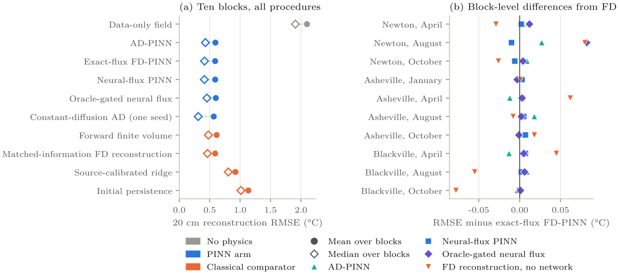
The operator variants have similar mean errors, and the gated variant has higher mean error. Table 2 gives equal-block means and medians of the within-block seed-mean RMSE, Table 3 the paired contrasts and Appendix 10 every block. The neural-flux arm has higher mean error than exact FD (0.591 against 0.590 °C) and the gated arm higher than raw neural flux (0.601). The matched-information numerical reconstruction, with no network, equals FD at 0.590 in a twentieth of a second. Lowest of all among complete procedures is the constant-diffusion AD ablation at 0.567, which motivates a separate assessment of the prescribed moisture multiplier.
| Method | Mean RMSE | Median RMSE | Mean seconds |
|---|---|---|---|
| Data-only field | 2.099 | 1.909 | 0.95 |
| AD-PINN | 0.594 | 0.430 | 6.05 |
| Exact-flux FD-PINN | 0.590 | 0.415 | 7.25 |
| Neural-flux PINN | 0.591 | 0.413 | 8.25 |
| Oracle-gated neural flux | 0.601 | 0.455 | 8.97 |
| Constant-diffusion AD (seed 11) | 0.567 | 0.312 | 5.25 |
| Forward finite volume | 0.615 | 0.479 | 0.04 |
| Matched-information FD reconstruction | 0.590 | 0.463 | 0.05 |
| Source-calibrated ridge | 0.924 | 0.806 | 0.00 |
| Initial persistence | 1.136 | 1.014 | 0.00 |
| Comparison | Mean difference | 95 % interval | Lower-error blocks |
|---|---|---|---|
| Neural flux FD | [0.0049, 0.0047] | 3/10 | |
| Gated neural flux | [0.0042, 0.0375] | 5/10 | |
| Neural flux AD | [0.0179, 0.0053] | 5/10 | |
| Gated FD | [0.0005, 0.0327] | 2/10 | |
| AD (seed 11) constant AD (seed 11) | [0.1305, 0.2444] | 3/10 |
At 0.0013 °C the primary difference has an interval spanning zero; the neural arm has lower error in three of ten blocks (two strictly at the printed precision, one tie). Only the gated-minus-FD interval excludes zero, favouring exact FD. The bootstrap is limited to three stations and one winter block.
6.2 Visited inputs, gradients and gate acceptance
Audits after Adam updates 0, 100, …, 700 save field weights, collocation coordinates and face inputs for every neural-flux and gated fit, and post-fit diagnostics use a new grid. The mean fraction of faces inside teacher support rounds to 0.999 and oracle-gate acceptance to 0.823 in both families. The raw learned-minus-exact spatial-operator RMS discrepancy averages 0.025 °C/day. Gated maxima are 0.0969 on neural-flux states and 0.0975 on gated states, inside the 0.10 °C/day budget of Equation 4 on every sampled state. That comparison holds the field fixed under two operators; it does not show the gated field is closer to the measured target, and a thresholded objective can change the optimiser’s trajectory even when every selected value meets its budget. A spacing ladder on each saved field, without refitting, measures the amplification channel: face errors enter the divergence over , but changing also changes the face inputs, so the ladder need not scale as .
6.3 Parameter-gradient audit
After the outcomes were known, an additional diagnostic was applied to all 60 neural-flux and gated fits (480 training snapshots and 60 final states) without refitting or changing any score or threshold. At each identical state the exact-FD, neural-flux and gated objectives were differentiated with respect to the field parameters , with data and initial terms identical and the gate at a fixed branch, and the relative discrepancy recorded with absolute differences and cosines (Table 4). On neural-flux states the gate lowers the median full-objective discrepancy from 1.207 % to 0.508 % and raises the median cosine from 0.999936 to 0.999989: closer sampled gradient agreement with FD at fixed states, and no explanation of why the separately optimised gated arm has higher error. Separating adaptive updates, trajectory effects, branch switching and model mismatch needs a different experiment.
| State family | Comparison | Median (%) | 95th percentile (%) | Median cosine |
|---|---|---|---|---|
| Neural flux | neural flux FD | 1.207 | 3.392 | 0.999936 |
| Neural flux | gated FD | 0.508 | 1.434 | 0.999989 |
| Gated | neural flux FD | 1.211 | 3.506 | 0.999936 |
| Gated | gated FD | 0.491 | 1.363 | 0.999989 |
6.4 Residuals, repeatability and cost
Mean new-grid continuous residual RMS values are 4.330 (AD), 4.226 (FD), 4.146 (gated) and 4.133 (neural flux) °C/day. They describe remaining equation mismatch under the assumed model, share the trained field, equation and AD library, and certify nothing physical. For neural-flux fields the discrete-operator discrepancy of about 0.025 and the continuous residual of about 4.133 are different quantities and do not partition fitting from physical error. A fresh Python process repeated all five seed-11 fits for the first eligible block with a maximum RMSE difference of 0 against a frozen tolerance of . The gate performs exact-map and Jacobian checks online, so no acceleration is inferred; any cost claim must include offline fitting, amortisation, guard overhead, inference and accuracy on controlled hardware.
7 Discussion
The matched-field comparison isolates the spatial operator and shows similar mean reconstruction errors. Neural flux, FD and AD sit within 0.004 °C of each other, and the gate adds 0.01 °C. A sparse linear reconstruction with the same information matches the exact-flux PINN at the reported precision. Improvement over the data-only field does not establish an advantage over the conventional reconstruction.
Jointly non-linear in moisture and temperature difference, the learned map approximates an oracle that is linear in the difference given moisture, so the generic odd approximation can introduce deviations from that conditional structure, and its held-out box error does not determine behaviour on fitted-field states outside the sampled moisture range. The input, Jacobian and fixed-state gradient audits probe possible perturbations without identifying a cause. Oracle access is at once the guard’s experimental strength and its practical limit. Exact values permit a transparent rejection test and an evaluated budget, and they also remove the reason to replace the operator. An oracle-free successor needs a separately justified enclosure and must be scored on new windows, since these targets have now informed interpretation.
Physical-model uncertainty is separate. The shape parameters were not measured at each site, the constant heat capacity is an approximation, and the Asheville winter block may involve omitted processes; the constant-diffusion ablation checks one choice and the fact that it scores best is a reason to revisit the multiplier before revisiting the operator. The study establishes no coupled hydrothermal dynamics, Caribbean transfer, forecast skill or projection. What it does supply is evidence about local coupling, residual design and reproducible evaluation for any face-flux architecture, and a reminder that a satisfied operator budget is not a solution certificate.
8 Conclusion
On these ten blocks a learned moisture-to-flux map does not improve the exact-FD PINN, and an oracle-assisted gate does not improve the learned map, while the gate’s evaluated budget is met everywhere it was sampled. The frozen protocol, before-scoring controls, retained snapshots, matched-information comparator and fresh-process repeat make the scope of that conclusion inspectable. The pointwise budget bounds the evaluated operator error, not the reconstruction error.
A Coverage register
Requested start dates were 20 January, 15 April, 15 August and 15 October 2024 at four stations. Eligible blocks: Newton 15 April, 15 August, 16 October (12:00); Asheville 20 January, 15 April, 15 August, 16 October (16:00); Blackville 15 April, 15 August, 15 October. Unavailable: Newton January; all four Crossville dates; Blackville January. Each eligible block supplies 96 hourly records and 95 scored targets.
B All block comparisons
| Block | AD | FD | Neural flux | Gated | Numerical reconstruction |
|---|---|---|---|---|---|
| GA Newton 8 W, April | 0.261 | 0.257 | 0.259 | 0.269 | 0.228 |
| GA Newton 8 W, August | 0.436 | 0.409 | 0.399 | 0.491 | 0.489 |
| GA Newton 8 W, October | 0.337 | 0.328 | 0.322 | 0.332 | 0.302 |
| NC Asheville 8 SSW, January | 0.366 | 0.366 | 0.369 | 0.363 | 0.367 |
| NC Asheville 8 SSW, April | 0.725 | 0.737 | 0.740 | 0.740 | 0.799 |
| NC Asheville 8 SSW, August | 0.354 | 0.336 | 0.341 | 0.338 | 0.328 |
| NC Asheville 8 SSW, October | 0.425 | 0.420 | 0.427 | 0.419 | 0.438 |
| SC Blackville 3 W, April | 1.061 | 1.074 | 1.081 | 1.079 | 1.119 |
| SC Blackville 3 W, August | 0.912 | 0.903 | 0.905 | 0.909 | 0.848 |
| SC Blackville 3 W, October | 1.061 | 1.064 | 1.064 | 1.065 | 0.986 |
Data and code availability
USCRN hourly files are public. The archive (protocol and configuration hashes, teacher and field weights, the 480 training snapshots, audit grids, score tables and the control-chain outputs) is held by the author and is available on request.
References
[1] Maziar Raissi, Paris Perdikaris, and George Em Karniadakis. Physics informed deep learning (Part I): Data-driven solutions of nonlinear partial differential equations. arXiv:1711.10561, 2017.
[2] Maziar Raissi, Paris Perdikaris, and George Em Karniadakis. Physics-informed neural networks: A deep learning framework for solving forward and inverse problems involving nonlinear partial differential equations. Journal of Computational Physics, 378: 686–707, 2019. doi: 10.1016/j.jcp.2018.10.045.
[3] Sanket Jantre, Deepak Akhare, Zhiyuan Wang, Xiaoning Qian, and Nathan M. Urban. Data-augmented few-shot neural emulator for computer-model system identification. arXiv:2508.19441, 2025.
[4] Yohai Bar-Sinai, Stephan Hoyer, Jason Hickey, and Michael P. Brenner. Learning data-driven discretizations for partial differential equations. Proceedings of the National Academy of Sciences, 116 (31): 15344–15349, 2019. doi: 10.1073/pnas.1814058116.
[5] Suryanarayana Maddu, Dominik Sturm, Bevan L. Cheeseman, Christian L. Müller, and Ivo F. Sbalzarini. STENCIL-NET for equation-free forecasting from data. Scientific Reports, 13: 12787, 2023. doi: 10.1038/s41598-023-39418-6.
[6] Pao-Hsiung Chiu, Jian Cheng Wong, Chinchun Ooi, My Ha Dao, and Yew-Soon Ong. CAN-PINN: A fast physics-informed neural network based on coupled-automatic-numerical differentiation method. Computer Methods in Applied Mechanics and Engineering, 395: 114909, 2022. doi: 10.1016/j.cma.2022.114909.
[7] Ramansh Sharma and Varun Shankar. Accelerated training of physics-informed neural networks (PINNs) using meshless discretizations. In Advances in Neural Information Processing Systems 35 (NeurIPS), 2022.
[8] Pranav Sunil and Ryan B. Sills. FE-PINNs: finite-element-based physics-informed neural networks for surrogate modeling. arXiv:2412.07126, 2024.
[9] Han Gao, Luning Sun, and Jian-Xun Wang. PhyGeoNet: Physics-informed geometry-adaptive convolutional neural networks for solving parameterized steady-state PDEs on irregular domain. Journal of Computational Physics, 428: 110079, 2021. doi: 10.1016/j.jcp.2020.110079.
[10] Stavros C. Kassinos. Auxiliary finite-difference residual-gradient regularization for PINNs. Machine Learning for Computational Science and Engineering, 2: 25, 2026. doi: 10.1007/s44379-026-00076-w.
[11] Yanling Wang, Liangsheng Shi, Xiaolong Hu, Wenxiang Song, and Lijun Wang. Multiphysics-informed neural networks for coupled soil hydrothermal modeling. Water Resources Research, 59 (1): e2022WR031960, 2023. doi: 10.1029/2022WR031960.
[12] Ali Reza Sepaskhah and Maasumeh Mazaheri-Tehrani. A sigmoidal model for predicting soil thermal conductivity-water content function in room temperature. Scientific Reports, 14, 2024. doi: 10.1038/s41598-024-68455-y.
[13] Aditi S. Krishnapriyan, Amir Gholami, Shandian Zhe, Robert M. Kirby, and Michael W. Mahoney. Characterizing possible failure modes in physics-informed neural networks. In Advances in Neural Information Processing Systems 34 (NeurIPS), 2021. arXiv:2109.01050.
[14] Sifan Wang, Yujun Teng, and Paris Perdikaris. Understanding and mitigating gradient flow pathologies in physics-informed neural networks. SIAM Journal on Scientific Computing, 43 (5): A3055–A3081, 2021. doi: 10.1137/20M1318043.
[15] Sifan Wang, Xinling Yu, and Paris Perdikaris. When and why PINNs fail to train: A neural tangent kernel perspective. Journal of Computational Physics, 449: 110768, 2022. doi: 10.1016/j.jcp.2021.110768.
[16] Tim De Ryck, Florent Bonnet, Siddhartha Mishra, and Emmanuel de Bézenac. An operator preconditioning perspective on training in physics-informed machine learning. In International Conference on Learning Representations (ICLR), 2024. arXiv:2310.05801.
[17] Jeremy Yu, Lu Lu, Xuhui Meng, and George Em Karniadakis. Gradient-enhanced physics-informed neural networks for forward and inverse PDE problems. Computer Methods in Applied Mechanics and Engineering, 393: 114823, 2022. doi: 10.1016/j.cma.2022.114823.
[18] Siddhartha Mishra and Roberto Molinaro. Estimates on the generalization error of physics-informed neural networks for approximating PDEs. IMA Journal of Numerical Analysis, 43 (1): 1–43, 2023. doi: 10.1093/imanum/drab093.
[19] NOAA National Centers for Environmental Information. U.S. climate reference network hourly files: format and data-field documentation; 2023–2024 hourly observations for GA newton 8 w, NC asheville 8 ssw, SC blackville 3 w and TN crossville 7 nw. https://www.ncei.noaa.gov/pub/data/uscrn/products/hourly02/, 2026. Accessed October 2026.