Keywords: Caribbean; heavy rainfall; thermodynamic features; geographic transfer; probabilistic verification; reanalysis; Brier score.
1 Introduction
Physics can enter a machine-learning model through governing equations, hard constraints, loss penalties or a transformation of the predictors, and these routes do not carry the same guarantees. Multi-variable hard constraints exist for downscaling [1, 2]; converting temperature and dew point into moisture variables provides nothing of the kind. This pilot isolates the smallest of these interventions, a coordinate change, and asks whether it improves next-day heavy-rain probabilities when the target cell is absent from model development. The primary comparison was fixed before outcomes were inspected, and the analysis retains null and adverse outcomes.
Regional studies motivate independent evaluation. Gridded-product evaluations against Caribbean gauges show that resolution and accuracy are not interchangeable [3, 4]; a calibrated Caribbean weather generator [5] and dynamical downscaling for Puerto Rico [6] are established baselines; and representing small islands as ocean at coarse resolution has documented consequences [7]. The NowcastNet evaluation [8] is instructive about aggregate-precipitation limits and is a different task at a different scale. Moisture predictors, boosting, blocked evaluation and cross-region transfer all have prior art, including a geographic downscaling benchmark [9]; the study combines them in one prespecified test.
2 Physical basis and hypothesis
Water vapour is necessary for heavy rain; it does not by itself determine ascent, condensation or rainfall efficiency. Tropical temperature-rainfall scaling reflects circulation and pre-rainfall cooling, with a Caribbean Sea example in the literature [10], and regional extremes relate to sea-surface temperature [11]; a fixed temperature multiplier is not a daily-rainfall law. The transformation uses the standard saturation-vapour-pressure approximation [12]: with , , temperatures in °C, and in hPa, the API pressure in kPa, and and in g kg. The relation is over liquid water and is a warm-surface diagnostic. Specific humidity computed from daily-mean dew point and pressure is only an approximation to the daily-mean specific humidity, because the map is non-linear; neither nor is column water, moisture convergence or precipitation, and no budget closure is imposed.
Under the hypothesis being tested, replacing with lowers held-out Brier score relative to an otherwise matched classifier. A monotonic variant constrains the fitted response to increase with at fixed remaining inputs; this is a contestable prior, since higher surface moisture does not compel more rain and holding fixed while varying changes the implied thermal state, so it cannot be called enforcement of a physical law.
3 Data and design
3.1 Provenance
Six point requests to the NASA POWER daily API (version 2.10.1) at Jamaica (18.1, 77.3), Cuba (21.5, 79.5), Hispaniola (19.0, 71.0), Puerto Rico (18.2, 66.5), Barbados (13.15, 59.55) and Trinidad (10.5, 61.3) returned corrected precipitation, 2 m temperature, 2 m dew or frost point, surface pressure and 2 m wind speed, with MERRA-2 and POWER as reported sources [13, 14]. Each series has 16,071 daily records from 1 January 1981 to 31 December 2024, no missing values and no physical-screen failures; dropping the first temperature-difference row and the last unavailable target leaves 16,069 examples per cell, 96,414 in all. The labels name the requested points; they are neither island averages nor a sample of islands, since the six were chosen deliberately. At the native resolution of a small island occupies part of a cell. Predictors and target originate in the same reanalysis, whose corrected land precipitation itself uses observational information [15]; any later gauge comparison must audit that dependence.
3.2 Target, information set and splits
For predictor day the target is , a study event definition rather than a validated flood threshold; 10 and 30 mm/day are exploratory sensitivities. All meteorological predictors are from day or earlier and the seasonal encoding uses the target date. Training uses target dates through 2005, calibration 2006–2010 and evaluation 2011–2024. In the temporal design each model uses its own cell’s earlier records; in the transfer design the whole target cell is excluded from training and calibration and the other five cells supply development data, with no coordinates or cell identifiers as features [16]. Because final reanalysis arrives after the represented time, the task is retrospective one-day-ahead inference under an assumed available day- state, and an operational forecast would need a different input stream.
3.3 Models, calibration and scoring
The raw feature vector has eight components: annual sine and cosine, , , , wind speed, and . The thermodynamic vector replaces the two temperatures with and , so the two representations have equal dimensionality and the same information source. The family comprises seasonal logistic regression; seasonal plus rainfall-lag logistic; full raw and moisture logistic; raw and moisture histogram gradient boosting [17]; a monotonic moisture boosting; and a shuffled-label raw boosting control that permutes training outcomes within cell and month, which keeps seasonal information and breaks the daily pairing. Logistic models use training-only standardisation, and 1,000 iterations; boosting uses 100 iterations, learning rate 0.07, at most seven leaves, at least 60 samples per leaf and regularisation 1, without early stopping or any parameter search. Each model receives a logistic calibration fitted on the calibration period only. There are fitted base models and as many calibration fits; a fresh execution reproduces all 576 metric rows exactly.
Brier score [18, 19], averaged equally across cells, is the primary metric; log loss, average precision (read against prevalence) and ROC AUC are secondary. The primary estimand is the equal-cell Brier difference between moisture and raw boosting in the transfer design. Paired bootstrap samples resample complete test years jointly across all six cells, 2,000 draws, recomputing the within-cell differences and their equal-cell mean; the percentile interval conditions on the fitted models and the chosen cells and excludes training-sample, model-selection and regional-sampling uncertainty. A seven-day-block sensitivity and a leave-one-cell-out summary are archived.
4 Results
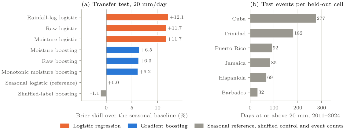
Per cell the transfer test has 5,114 days, giving 30,684 cell-days and 737 exceedances, a pooled prevalence of 2.402 %: Cuba 277, Trinidad 182, Puerto Rico 92, Jamaica 85, Hispaniola 69 and Barbados 32. These are reanalysis-cell exceedances and their spread is why a pooled score alone is inadequate.
The primary comparison fails its criterion. Moisture boosting has a mean Brier score of 0.021933 against 0.021968 for raw boosting (Table 1), a relative reduction of about 0.16 %; the paired difference is and both the year-block interval, , and the seven-day-block interval cross zero. Five of six cells show a decrease, and the archived leave-one-cell-out summary shows the mean changing sign when influential cells are excluded.
The rainfall-lag logistic baseline has the lowest Brier score, 0.020614, which is 12.1 % below the seasonal logistic baseline (0.023451), and the best log loss, average precision and AUC. Adding the remaining raw variables does not improve it (0.020710), so neither more variables nor more model capacity explains the skill that exists here.
Three sensitivity analyses qualify the result. The monotonic moisture model is worse than raw boosting at the primary threshold (0.022002) and at 10 mm/day its exploratory interval lies above zero, an adverse sensitivity that argues against treating a monotone moisture response as an automatically beneficial constraint. The shuffled-label control (0.023712) sits near the seasonal baseline (0.023451), as it should. In the temporal design moisture boosting moves the mean Brier score from 0.022034 to 0.021941, again with an interval including zero; at 10 and 30 mm/day the transfer differences have different signs with intervals spanning zero. Sensitivities were run without multiplicity correction and stay exploratory.
| Model | Brier | Log loss | Avg. precision | ROC AUC |
|---|---|---|---|---|
| Seasonal logistic | 0.023451 | 0.113707 | 0.0324 | 0.6298 |
| Rainfall-lag logistic | 0.020614 | 0.083758 | 0.1785 | 0.8688 |
| Raw logistic | 0.020710 | 0.084790 | 0.1763 | 0.8687 |
| Moisture logistic | 0.020717 | 0.084870 | 0.1770 | 0.8687 |
| Raw boosting | 0.021968 | 0.090724 | 0.1578 | 0.8605 |
| Moisture boosting | 0.021933 | 0.090677 | 0.1635 | 0.8583 |
| Monotonic moisture boosting | 0.022002 | 0.091045 | 0.1610 | 0.8587 |
| Shuffled-label boosting | 0.023712 | 0.121855 | 0.0370 | 0.6466 |
5 Discussion
In this experiment the coordinate change does not establish improved transfer skill. Moisture remains physically relevant; the test concerns whether its diagnostic representation adds statistical structure beyond the raw variables at this model budget, and a non-linear transformation can change how finite trees partition the space without adding information. Three explanations remain open, and the pilot cannot separate them. The raw variables may already carry the moisture signal. Surface humidity may represent column moisture and lifting poorly. A calibration learned on five cells may not transfer to a sixth.
The rainfall-lag baseline supports testing persistence and calibration before increasing model complexity. It does not show that a logistic model is optimal. No hyperparameter search, neural network or numerical comparison was run, and a tuned ensemble, a longer history or circulation predictors might change the ranking. Any such follow-up needs a new evaluation period, since this holdout has now been inspected. The pilot is an ablation for a later, stronger test: one of water-budget or transport constraints on dense fields, with physical residuals and independent rainfall skill scored separately. That test must keep two things apart. Coarse-to-fine consistency is not conservation of the water budget, and an attractive reconstructed field is not improved extremes [20].
6 Limitations and the next experiment
Predictors and targets share one reanalysis origin, and that is the principal limitation: the result is a statistical relationship inside that system. Six purposive cells cannot characterise islands, elevation bands or coastlines, and a coarse-cell daily total cannot resolve sub-hourly flash-flood extremes. Barbados has 32 events, too few for a cell-level verdict. Reanalysis latency rules out operational use at the assumed issue time, and no NWP hindcast was compared. The bootstrap interval conditions on the fitted models and fourteen test years; it neither establishes equivalence nor excludes a modest benefit. One boosting configuration was tested, the monotonic prior is heuristic, and pooled reliability can hide cell-level calibration errors. The confirmatory experiment pairs dense Caribbean precipitation fields with independently audited gauges, retains whole-island and whole-event holdouts, documents release times, compares against an archived NWP hindcast, and separates feature transformations from enforced physical identities. Two gridded products alone cannot establish ground truth, so the independence of any gauge set from the reference has to be audited; CHIRPS [21] is a candidate reference whose gauge blending makes that audit essential.
7 Conclusion
In six Caribbean reanalysis cells, a moisture-based feature representation produces a small, uncertain change in next-day heavy-rain probability skill and does not outperform the simplest competitive baseline. The results support retaining rainfall-persistence baselines and strict transfer evaluation in later physics-informed studies. A forecasting improvement, a general failure of physics-informed learning and a validated warning system are all claims this experiment leaves unsupported.
Data and code availability
NASA POWER daily data are public. The research package (API responses, feature code, the 288 fitted models and calibrations, the 576 metric rows, bootstrap draws and the leave-one-cell-out and seven-day-block sensitivities) is held in the author’s archive and is available on request.
References
[1] Jose González-Abad, Jorge Baño-Medina, and José Manuel Gutiérrez. Multi-variable hard physical constraints for climate model downscaling. arXiv:2308.01868, 2023.
[2] Paula Harder, Alex Hernandez-Garcia, Venkatesh Ramesh, Qidong Yang, Prasanna Sattegeri, Daniela Szwarcman, Campbell Watson, and David Rolnick. Hard-constrained deep learning for climate downscaling. Journal of Machine Learning Research, 24 (365): 1–40, 2023. https://www.jmlr.org/papers/v24/23-0158.html.
[3] Abel Centella-Artola, Arnoldo Bezanilla-Morlot, Michael A. Taylor, Dimitris A. Herrera, Daniel Martín-Serrano, Maibys Sierra-Lorenzo, Alejandro Vichot-Llano, Jesús Cabrales-Infante, Jayaka D. Campbell, and Tannecia S. Stephenson. Evaluation of sixteen gridded precipitation datasets over the Caribbean region using gauge observations. Atmosphere, 11 (12): 1334, 2020. doi: 10.3390/atmos11121334.
[4] Ralph Bathelemy, Pierre Brigode, Dominique Boisson, and Emmanuel Tric. Rainfall in the Greater and Lesser Antilles: Performance of five gridded datasets on a daily timescale. Journal of Hydrology: Regional Studies, 43: 101203, 2022. doi: 10.1016/j.ejrh.2022.101203.
[5] P. D. Jones, C. Harpham, A. Burton, and C. M. Goodess. Downscaling regional climate model outputs for the Caribbean using a weather generator. International Journal of Climatology, 36 (12): 4141–4163, 2016. doi: 10.1002/joc.4624.
[6] Jared H. Bowden, Adam J. Terando, Vasu Misra, Adrienne Wootten, Amit Bhardwaj, Ryan Boyles, William Gould, Jaime A. Collazo, and Tanya L. Spero. High-resolution dynamically downscaled rainfall and temperature projections for ecological life zones within Puerto Rico and for the U.S. Virgin Islands. International Journal of Climatology, 41 (2): 1305–1327, 2021. doi: 10.1002/joc.6810.
[7] Philippe Cantet, Michel Déqué, Philippe Palany, and Jean-Louis Maridet. The importance of using a high-resolution model to study the climate change on small islands: the Lesser Antilles case. Tellus A: Dynamic Meteorology and Oceanography, 66: 24065, 2014. doi: 10.3402/tellusa.v66.24065.
[8] Puja Das, August Posch, Nathan Barber, Michael Hicks, Kate Duffy, Thomas Vandal, Debjani Singh, Katie van Werkhoven, and Auroop R. Ganguly. Hybrid physics-AI outperforms numerical weather prediction for extreme precipitation nowcasting. npj Climate and Atmospheric Science, 7: 282, 2024. doi: 10.1038/s41612-024-00834-8.
[9] Paula Harder, Luca Schmidt, Francis Pelletier, et al. Benchmarking the geographic generalization of deep learning models for precipitation downscaling. Scientific Reports, 2026. doi: 10.1038/s41598-025-34557-4.
[10] Dominik Traxl, Niklas Boers, Aljoscha Rheinwalt, and Bodo Bookhagen. The role of cyclonic activity in tropical temperature-rainfall scaling. Nature Communications, 12: 6732, 2021. doi: 10.1038/s41467-021-27111-z.
[11] Carlo Destouches, Arona Diedhiou, Sandrine Anquetin, Benoit Chanzy, Adermus Joseph, Nathan Pierre, and Adrien Dumont. Changes in extreme precipitation patterns over the Greater Antilles and teleconnection with large-scale sea surface temperature. Earth System Dynamics, 16: 497–530, 2025. doi: 10.5194/esd-16-497-2025.
[12] David Bolton. The computation of equivalent potential temperature. Monthly Weather Review, 108 (7): 1046–1053, 1980. doi: 10.1175/1520-0493(1980)108<1046:TCOEPT>2.0.CO;2.
[13] NASA POWER. Data sources, energy-flux methodology and daily API documentation. https://power.larc.nasa.gov/docs/methodology/, 2026. Accessed 14 October 2026. Retrieved headers identify CERES SYN1deg as the radiation source.
[14] Ronald Gelaro, Will McCarty, Max J. Suárez, et al. The Modern-Era Retrospective Analysis for Research and Applications, version 2 (MERRA-2). Journal of Climate, 30 (14): 5419–5454, 2017. doi: 10.1175/JCLI-D-16-0758.1.
[15] Rolf H. Reichle, Q. Liu, Randal D. Koster, Clara S. Draper, Sarith P. P. Mahanama, and Gary S. Partyka. Land surface precipitation in MERRA-2. Journal of Climate, 30 (5): 1643–1664, 2017. doi: 10.1175/JCLI-D-16-0570.1.
[16] David R. Roberts, Volker Bahn, Simone Ciuti, Mark S. Boyce, Jane Elith, Gurutzeta Guillera-Arroita, Severin Hauenstein, José J. Lahoz-Monfort, Boris Schröder, Wilfried Thuiller, David I. Warton, Brendan A. Wintle, Florian Hartig, and Carsten F. Dormann. Cross-validation strategies for data with temporal, spatial, hierarchical, or phylogenetic structure. Ecography, 40 (8): 913–929, 2017. doi: 10.1111/ecog.02881.
[17] Jerome H. Friedman. Greedy function approximation: A gradient boosting machine. The Annals of Statistics, 29 (5): 1189–1232, 2001. doi: 10.1214/aos/1013203451.
[18] Glenn W. Brier. Verification of forecasts expressed in terms of probability. Monthly Weather Review, 78 (1): 1–3, 1950. doi: 10.1175/1520-0493(1950)078<0001:VOFEIT>2.0.CO;2.
[19] Tilmann Gneiting and Adrian E. Raftery. Strictly proper scoring rules, prediction, and estimation. Journal of the American Statistical Association, 102 (477): 359–378, 2007. doi: 10.1198/016214506000001437.
[20] P. Jyoteeshkumar Reddy, Richard Matear, John Taylor, et al. Limitation of super-resolution machine learning approach to precipitation downscaling. Scientific Reports, 2025. doi: 10.1038/s41598-025-05880-7.
[21] Chris Funk, Pete Peterson, Martin Landsfeld, Diego Pedreros, James Verdin, Shraddhanand Shukla, Gregory Husak, James Rowland, Laura Harrison, Andrew Hoell, and Joel Michaelsen. The climate hazards infrared precipitation with stations: a new environmental record for monitoring extremes. Scientific Data, 2: 150066, 2015. doi: 10.1038/sdata.2015.66.