Keywords: physics-informed neural networks; precipitation nowcasting; model discrepancy; finite-volume methods; identifiability; conservation.
1 Introduction
Das et al. evaluated NowcastNet [1] against HRRR, persistence and advection over 30 heavy-precipitation events in the Tennessee Valley [2]. The comparison is a useful motivation and a bounded one. Their results section reports that advection can have better probability of detection and that HRRR can be better on continuous error at two- and three-hour leads; over-estimation grows with lead; and the image-evolution relation in their methods, motion plus an intensity residual, is an effective equation for a rain-rate picture, not a water budget. A rain-rate image is a picture of a flux, and a learned source on that picture identifies neither condensation nor a moisture transport on its own.
The question this paper asks is narrower than “does physics help”. At matched observations, architecture and compute, does a development-calibrated closure tolerance improve held-out precipitation prediction relative to an incorrectly rigid physical prior and a validation-tuned soft penalty, while keeping non-negativity and numerical balance? The estimand is the paired difference in a prespecified event-level score. The name CLEAR-PINN (closure-limited, evidence-adaptive residual physics-informed neural network) identifies the formulation; it does not claim that correction-aware physics-informed learning is new, since misspecification-aware PINNs [3], conservative domain decomposition [4] and physics-embedded nowcasters already exist. The formulation specifies the admissible correction, observation support and numerical ledger. The evaluation protocol defines the evidence needed to support or reject the design. The paper presents four contributions: the formulation itself (Section 4); four elementary propositions that bound what it can promise, each checked numerically (Section 5); a synthetic component experiment whose negative result on the adaptive tolerance is kept (Section 6); and the evaluation protocol under which the design is to be accepted or rejected (Section 7).
2 Related work: why stronger physics is insufficient
Classical PINNs combine data, boundary conditions and equation residuals [5], and their optimisation can fail even when the equation is right [6, 7]; causal training, domain decomposition and local bases address parts of this [8, 9, 10]. Residual-adaptive sampling [11] and variational forms [12] change how equation information is used, but a large residual need not mark a region where the nominal equation is trustworthy; it may mark an omitted process or a sensor artefact, and a sampler that concentrates there enforces the wrong thing harder. Neural operators [13] are a candidate amortised backbone, not an accuracy result, and a finite-element comparison [14] is a reminder that a conventional solver on the same budget is the baseline to beat. Bayesian PINNs [15] treat uncertainty but not the identifiability of a learned source against a learned motion. Recent coarse-graining work [16] examines which constraints survive aggregation under specified filtering assumptions. Those assumptions must be checked for the chosen rain-image model.
3 Quantities and observation model
Let be a cell-averaged rain rate in mm h−1 on a horizontal domain. The effective image model is (1) with an effective pattern velocity, an initiation term and a growth or decay rate. The advective form differs by ; treating the two as interchangeable moves a divergence term into the source without recording it. The column-water budget (2) is a separate relation in separate units (kg m−2 and kg m−2 s−1); a balance for Equation 1 cannot establish Equation 2, and no atmospheric-water observation enters the experiment below. Each product observes through its own operator, , with support, averaging, mask and retrieval made explicit; missing observations are masked and never set to zero rain. The initial state uses only information available at issue time, and lateral boundaries are prescribed inflow, an open-boundary rule or a stated closed domain, never silently periodic in a geographical run.
4 Formulation
4.1 Conservative transport and bounded reaction
Partition the domain into cells of area . For a shared internal face between cells and with length and outward normal velocity , the first-order upwind flux is with and , and . The transport substep is (3) One velocity and one flux are used per shared face. Two independently predicted outward fluxes would generally prevent exact cancellation. The closure head predicts bounded and , held fixed during the exact affine reaction substep (4) The exact substep removes the explicit-reaction positivity restriction; it does not make the split solution exact. The executed prototype sets and learns only a signed growth field, which rules out rain appearing in a dry cell and leaves initiation to a later experiment.
4.2 Three residuals that must stay separate
With the integrated effective source , the algebraic ledger (5) vanishes to arithmetic error whenever the update is implemented correctly. It is an implementation check; penalising it gives no training signal. With an independently specified nominal source (possibly zero), the nominal residual (6) measures departure from a source prior. A third quantity, the column-water residual from Equation 2, exists only when its variables are observed. A model can pass the first and fail both others, and the three must be reported separately.
4.3 Evidence-adaptive tolerance
The proposed nominal-relation loss is (7) with an area weight, an evidence-support weight, a scale and a tolerance. Inside the band the nominal prior exerts no force; outside it the penalty grows quadratically. Tolerance and support rule are estimated on training sequences, selected on validation events and frozen before testing. They come from weak source residuals of historical sequences under a separately estimated motion field and the stated observation operator, stratified by regime indicators, with a resistant residual envelope and a pooled fallback for sparse strata. The forecasting network is prohibited from adjusting or jointly with the forecast loss, since that would be a direct route to disabling the constraint; sensitivity runs must still cover , pooled and regime-dependent tolerances, and deliberately inflated tolerances, the last of which approaches an unconstrained closure and measures whether the nominal physics contributes anything beyond architecture. Observation availability does not establish the adequacy of the equation. A well-observed cell can violate an incomplete equation, and the support weight records evidence availability rather than a low model residual.
4.4 Objective, architecture and compute
A full objective is , with the last term used only when an independent moisture relation is available, every term scaled to dimensionless form on training statistics. An amortised encoder would ingest recent rain fields, masks, terrain and context and predict shared-face motion and bounded closure parameters; the solver advances the state. A probabilistic extension would pass every ensemble member through the same positive update, since adding image noise after the solver bypasses its guarantees. The present prototype has no encoder, no moisture head and no stochastic branch. The stencil cost of the transport step is linear in cell count; any adaptive refinement must keep one shared face flux and aggregate fine and coarse interface fluxes consistently; and the honest efficiency comparison includes spending the same time on a finer conventional solver.
5 Mathematical properties
Assumption 1. Cell averages and inflow states are non-negative; ; the transport step satisfies in every cell; closure parameters are finite and held fixed within a substep.
Proof. The transport state is times plus incoming contributions . The exponential factor is positive and for finite real . ◻
The result does not cover higher-order reconstructions, unrestricted neural fluxes, assimilation increments or post-processing, and bounded growth does not bound long-rollout error.
Proposition 2 (Domain ledger). For shared internal fluxes,
Proof. Multiply Equation 5 by and sum; each internal flux appears twice with opposite sign. ◻
With periodic or zero-flux boundaries and zero source the area-weighted intensity sum is preserved; with a source it changes by the recorded source. Whether the learned source is physically right is a separate question that the ledger leaves open.
Proposition 3 (Transport-source non-identifiability). For an unrestricted, sufficiently regular source and any field compatible with the boundary conditions, if satisfies Equation 1 then produces the same trajectory.
Proof. Substitute; the extra transport term is exactly the added source. ◻
Within the bounded affine class the ambiguity holds whenever both sources are admissible. Perfect rain observations cannot identify both fields; bounding the closure shrinks the admissible set without proving uniqueness, and in dry or flat regions the motion stays poorly determined. Independent motion estimates, multiple views or a defensible source model are needed before a learned velocity is read physically.
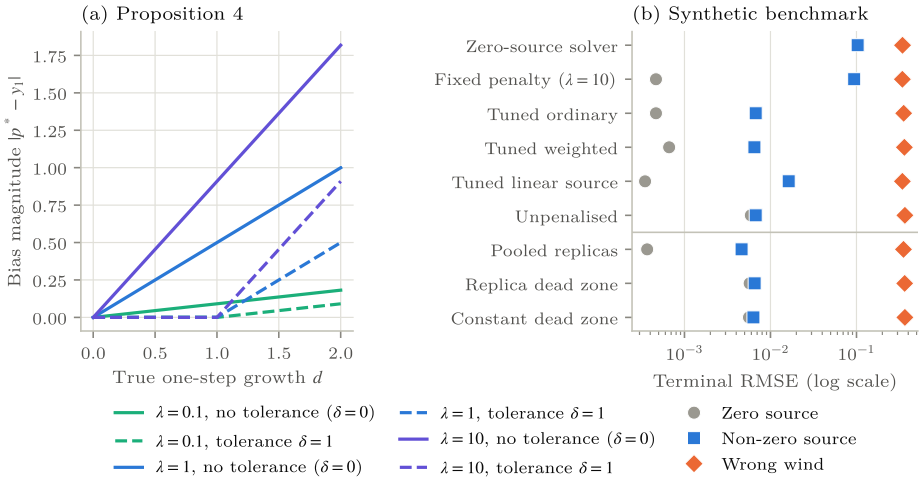
Proposition 4 (Bias from an incomplete source prior). For a scalar one-step observation with , , , the minimiser of satisfies if and otherwise, so the bias is .
Proof. Convexity places the minimiser between and ; inside the band the observation is unpenalised; outside, stationarity gives . ◻
With a stronger penalty pulls the prediction toward the wrong no-growth prior, and a tolerance at least removes the bias in this noiseless case. Nothing here is an optimal-tolerance theorem under noise. A large tolerance also admits spurious growth, which is why a zero-source control and a tuned ordinary penalty are needed.
6 Synthetic component experiment
6.1 Manufactured problem
All quantities are dimensionless. The state is 64 cell means on a periodic unit interval, , , 50 steps to , true velocity (Courant 0.32); the wrong-wind condition supplies to the forecast model (Courant 0.448). Simulator and forecaster share the upwind transport and multiplicative reaction with . The sourced simulator uses with a smooth random context field; the zero-source regime sets . Each of five seeds has 20 training, 8 validation and 20 test events per regime, test events generated after fitting and selection, with protocol, seeds and configuration hash saved beforehand. The 100 seed-event evaluations per regime are dependent within seed; they stand for five fitted models, each tested twenty times.
For a positive historical transition and the assumed velocity, plus Gaussian noise of standard deviation 0.25 is the training target. A second independent noisy replica of the same one-step coefficient defines the support weight , available only in training. That replica is not a temporally separate measurement, and it gives the weighted learner extra source-sensitive information the ordinary baseline does not see; Section 6.4 fixes this.
6.2 Comparators
The neural source has inputs , one hidden layer of 12 tanh units and a tanh output bounding . The ordinary family minimises mean squared source-target error plus ; the weighted family uses . Both use weight decay , the same initialisation per seed, chosen by mean terminal validation RMSE, and a 150-iteration L-BFGS-B cap. Other comparators are persistence, zero-source finite-volume transport, a strong fixed penalty , the unpenalised closure, a linear source with the same inputs clipped to , and an oracle with the simulator’s motion and source (zero error by construction). The weighted quadratic gate is a precursor of Equation 7 rather than its dead zone, so the primary run tests the weighting mechanism only.
6.3 Primary results and adverse controls
Allowing a source cuts terminal RMSE in the sourced regime from 0.103227 (zero-source solver) to 0.006736 (tuned ordinary neural) and 0.006508 (tuned weighted); Table 1. The weighted-minus-ordinary difference is with a 2,000-draw hierarchical bootstrap interval of : no benefit beyond ordinary validation-selected regularisation. In the zero-source control the exact solver wins and weighting raises neural error by with interval . Under wrong wind the weighted-minus-ordinary difference is with interval , and the strong fixed penalty and the linear source both beat the tuned neural families. That is the caution against reading the learned closure as physics. It compensates the wrong transport while the ledger stays at machine precision.
| Method | Zero source | Non-zero source | Wrong wind |
|---|---|---|---|
| Persistence | 0.635617 | 0.645967 | 0.645967 |
| Zero-source finite volume | 0.000000 | 0.103227 | 0.342793 |
| Strong fixed neural penalty () | 0.000466 | 0.094042 | 0.341274 |
| Validation-tuned ordinary neural | 0.000466 | 0.006736 | 0.353515 |
| Validation-tuned weighted neural | 0.000663 | 0.006508 | 0.360244 |
| Validation-tuned linear source | 0.000348 | 0.016282 | 0.341617 |
| Unpenalised neural source | 0.005907 | 0.006736 | 0.365248 |
| Oracle simulator | 0.000000 | 0.000000 | 0.000000 |
6.4 Matched-information and dead-zone tests
Two limits in the primary design became clear once it had run. The weighted penalty is not the proposed dead zone, and the weighted learner sees two replicas while its comparator sees one. Follow-up protocols were frozen before their own evaluation and are exploratory. The first fits with from the second replica, and a constant-budget control uses the median of those tolerances; both act on the coefficient, not on the dimensional residual of Equation 6. The second fits the ordinary quadratic network to , which is equivalent to fitting both replicas and gives the comparator the same two observations through a simpler rule.
Ordinary pooling is better than both adaptive rules in the sourced regime (Table 2). Dead-zone minus pooled is with interval , and weighted minus pooled with . In the zero-source control the dead-zone difference is with , a wider tolerance having disabled useful denoising of spurious source estimates. Under wrong wind it is with . The adaptive rules add no predictive value here. The result cannot show that the full dimensional rule always fails, but it demands a stronger calibration rationale before that complexity is added.
| Method | Zero source | Non-zero source | Wrong wind |
|---|---|---|---|
| Ordinary quadratic on pooled replicas | 0.000368 | 0.004612 | 0.351736 |
| Replica-weighted quadratic | 0.000663 | 0.006508 | 0.360244 |
| Replica-specific dead zone | 0.005723 | 0.006545 | 0.363192 |
| Constant dead zone | 0.005621 | 0.006336 | 0.365248 |
6.5 Numerical checks and the optimisation limit
All 120 logged primary neural fits reached the 150-iteration cap without meeting the optimiser’s convergence criterion; 15 reuse an identical zero-penalty fit, leaving 105 unique fits. All 120 dead-zone and 60 pooled records also reach the cap. These are budget-limited comparisons, not comparisons of converged optima, and equal caps are not equal wall-clock. Finite-difference checking of the hand-written gradient gave a maximum discrepancy of ; the minimum state over all forecasts was 0.048654; the largest local ledger defect was ; a repeated-step zero-source check drifted by . One hundred Courant-admissible cases and 100 scalar minimisers were checked against the propositions, and a deliberate Courant violation produced a state of . A fresh execution reproduced the event, lead, penalty and bootstrap CSVs byte for byte in about 53 seconds of CPU time; that figure records reproducibility on a small problem and says nothing about nowcasting speed.
7 Protocol for a meteorological evaluation
The proposed meteorological protocol specifies the comparisons needed to support or reject the design. The task is intensity and accumulation over a stated 0–3 h horizon with storm events as the primary unit, an operationally representative test set and a separately reported extreme subset. The first replication target is the Das et al. task where products, events and preprocessing can be obtained; a Caribbean study follows only after coverage, licensing and event independence are audited, and no Caribbean radar archive has been secured. Every input carries measurement time, issue time, arrival time, version, support and missingness; IMERG Early has a latency of about four hours [17], so a nominally contemporaneous field cannot be assumed at issue. Validating a gauge-adjusted product against its own gauges has to be declared as such, and reanalysis enters as an analysed product with its own error.
Splits are assigned before preprocessing with whole storms in one partition; training fits normalisation, envelopes, operators and regime indicators; validation selects hyperparameters; test holds untouched event blocks and at least one external region or season if transfer is claimed. No test event may be used to choose , the source cap, an illustration or an interval. Baselines are Eulerian persistence, an optical-flow or pySTEPS configuration [18], a numerical transport model, a statistical growth model, unconstrained machine learning, an accessible generative nowcaster [1, 19] and an issue-time-matched regional NWP archive. The central comparison holds encoder, solver, events and budget fixed and varies only the source-prior treatment: zero tolerance, tuned quadratic, unrestricted, pooled and regime-dependent tolerance, plus ablations that remove motion information, replace the network with a linear source, disable initiation and withhold optional inputs. Scores are event-level error, accumulation bias, a preselected extreme score (CSI, POD, FAR at declared thresholds), FSS and catchment accumulations, proper probabilistic scores [20] if a probabilistic head exists, the ledger, minimum intensity, nominal residual, source size and roughness, and full compute cost including tuning. Intervals resample storm blocks.
The method is supported only if it beats both the rigid prior and the tuned ordinary penalty on the frozen primary comparison without unacceptable false-alarm, positivity or latency cost, against a margin agreed with operational partners in advance. It is revised or rejected if the advantage disappears after penalty tuning, a linear source matches it at lower cost, the closure compensates wrong motion, tolerance inflation removes the effect, or skill depends on inputs unavailable at issue time. Exact accounting does not resolve these predictive failures. Table 3 lists the diagnostic failures any implementation must run.
| Test | Check | Failure interpretation |
|---|---|---|
| Shared-face cancellation | Internal fluxes sum with opposite signs | Bookkeeping inconsistent; physical reading premature |
| Zero source, closed boundary | Area-weighted sum constant to arithmetic error | Implementation error or unrecorded change |
| Non-zero reaction | Use the integrated increment | Apparent drift may be a mis-specified audit |
| Courant violation | Exceed the stated step | Positivity guarantee no longer applies |
| Exactly dry cell | With , zero stays zero | Restricted head cannot claim initiation |
| Wrong motion | Perturb velocity independently of source | Closure compensates transport; low ledger error does not resolve it |
| Oversized tolerance | Approach unrestricted source | Benefit may come from disabling the prior |
| Zero-source noisy control | Compare false growth after training | Excess freedom reduces denoising |
| Missing sensor | Apply recorded mask and support rule | Confident physical reading unsupported |
| Delayed products | Reconstruct arrival times | Unavailable fields invalidate the comparison |
| Simple source comparator | Fit a linear or low-rank closure | Neural complexity unsupported if matched at lower cost |
8 Discussion
The formulation specifies separate requirements for equations, observations and learned corrections. Balance is enforced structurally; the source is allowed to express unresolved evolution within bounds; the nominal prior is then challenged with a separately selected tolerance; and the ledger, the nominal residual and any moisture residual are reported apart, so a tautological residual is never presented as evidence. Proposition 4 explains why indiscriminately strengthening a source-free prior degrades prediction; Proposition 3 explains why adding a correction network is not enough, since velocity and source can trade off behind a good image fit. Observation-aware evaluation has to test whether extra measurements shrink that ambiguity rather than assume extra channels do.
The efficiency case is plausible and unproven. A numerical backbone with a small closure avoids learning transport from scratch and amortises over initial conditions, but the strongest comparison is often a plain scheme with a low-rank source, and efficiency has to be reported as an error-cost frontier that includes tuning. Adaptive computation needs an epistemic stopping rule as well. When error comes from missing physics or bad data, more residual evaluations will not help, and a falling nominal residual with rising held-out error is a failure signal.
The complete architecture has not been implemented. The executed experiments are one-dimensional, periodic, manufactured, with restricted source and motion; they contain no radar retrieval, convection, water storage, real boundary, latency, probabilistic calibration or generative nowcaster. The matched-information comparison favours ordinary pooling, so the adaptive rules currently lack evidence of incremental value. The literature assessment is targeted and a name search cannot establish novelty; the defensible claim is an integrated formulation with explicit identifiability and falsification requirements and narrow theoretical and synthetic evidence. Caribbean applicability requires the event-held-out meteorological comparison specified above. The present synthetic evidence does not establish regional performance.
9 Conclusion
The formulation separates an exactly balanced update, a bounded learned source and a tolerance-banded nominal relation, and four propositions fix what it can promise: conditional non-negativity, an exact ledger that carries no physical evidence, non-identifiability of velocity and source from the rain field alone, and a bias from an incomplete source prior that a tolerance removes. The synthetic experiment supports the bounded source, which cuts terminal error from 0.103 to 0.0067 when the simulator has one, and does not support the adaptive tolerance, which loses to an ordinary quadratic penalty given the same information. The design is therefore left as a falsifiable protocol, and its next step is the event-held-out meteorological comparison, run so that it can reject the method.
Data and code availability
The synthetic experiment is self-contained. The solver, closure networks, protocol file, configuration hash, seeds and the event, lead, penalty and bootstrap tables are held in the research package, which is available on request and re-executes in under a minute of CPU time. No meteorological data were used.
References
[1] Yuchen Zhang, Mingsheng Long, Kaiyuan Chen, Lanxiang Xing, Ronghua Jin, Michael I. Jordan, and Jianmin Wang. Skilful nowcasting of extreme precipitation with NowcastNet. Nature, 619: 526–532, 2023. doi: 10.1038/s41586-023-06184-4.
[2] Puja Das, August Posch, Nathan Barber, Michael Hicks, Kate Duffy, Thomas Vandal, Debjani Singh, Katie van Werkhoven, and Auroop R. Ganguly. Hybrid physics-AI outperforms numerical weather prediction for extreme precipitation nowcasting. npj Climate and Atmospheric Science, 7: 282, 2024. doi: 10.1038/s41612-024-00834-8.
[3] Zongren Zou, Xuhui Meng, and George Em Karniadakis. Correcting model misspecification in physics-informed neural networks (PINNs). Journal of Computational Physics, 505: 112918, 2024. doi: 10.1016/j.jcp.2024.112918.
[4] Ameya D. Jagtap, Ehsan Kharazmi, and George Em Karniadakis. Conservative physics-informed neural networks on discrete domains for conservation laws: Applications to forward and inverse problems. Computer Methods in Applied Mechanics and Engineering, 365: 113028, 2020. doi: 10.1016/j.cma.2020.113028.
[5] Maziar Raissi, Paris Perdikaris, and George Em Karniadakis. Physics-informed neural networks: A deep learning framework for solving forward and inverse problems involving nonlinear partial differential equations. Journal of Computational Physics, 378: 686–707, 2019. doi: 10.1016/j.jcp.2018.10.045.
[6] Sifan Wang, Yujun Teng, and Paris Perdikaris. Understanding and mitigating gradient flow pathologies in physics-informed neural networks. SIAM Journal on Scientific Computing, 43 (5): A3055–A3081, 2021. doi: 10.1137/20M1318043.
[7] Aditi S. Krishnapriyan, Amir Gholami, Shandian Zhe, Robert M. Kirby, and Michael W. Mahoney. Characterizing possible failure modes in physics-informed neural networks. In Advances in Neural Information Processing Systems 34 (NeurIPS), 2021. arXiv:2109.01050.
[8] Sifan Wang, Shyam Sankaran, and Paris Perdikaris. Respecting causality for training physics-informed neural networks. Computer Methods in Applied Mechanics and Engineering, 421: 116813, 2024. doi: 10.1016/j.cma.2024.116813.
[9] Ameya D. Jagtap and George Em Karniadakis. Extended physics-informed neural networks (XPINNs): A generalized space-time domain decomposition based deep learning framework for nonlinear partial differential equations. Communications in Computational Physics, 28 (5): 2002–2041, 2020. doi: 10.4208/cicp.OA-2020-0164.
[10] Ben Moseley, Andrew Markham, and Tarje Nissen-Meyer. Finite basis physics-informed neural networks (FBPINNs): a scalable domain decomposition approach for solving differential equations. Advances in Computational Mathematics, 49: 62, 2023. doi: 10.1007/s10444-023-10065-9.
[11] Chenxi Wu, Min Zhu, Qinyang Tan, Yadhu Kartha, and Lu Lu. A comprehensive study of non-adaptive and residual-based adaptive sampling for physics-informed neural networks. Computer Methods in Applied Mechanics and Engineering, 403: 115671, 2023. doi: 10.1016/j.cma.2022.115671.
[12] Ehsan Kharazmi, Zhongqiang Zhang, and George Em Karniadakis. hp-VPINNs: Variational physics-informed neural networks with domain decomposition. Computer Methods in Applied Mechanics and Engineering, 374: 113547, 2021. doi: 10.1016/j.cma.2020.113547.
[13] Zongyi Li, Nikola Kovachki, Kamyar Azizzadenesheli, Burigede Liu, Kaushik Bhattacharya, Andrew Stuart, and Anima Anandkumar. Fourier neural operator for parametric partial differential equations. In International Conference on Learning Representations (ICLR), 2021. arXiv:2010.08895.
[14] Tamara G. Grossmann, Urszula Julia Komorowska, Jonas Latz, and Carola-Bibiane Schönlieb. Can physics-informed neural networks beat the finite element method? IMA Journal of Applied Mathematics, 89 (1): 143–174, 2024. doi: 10.1093/imamat/hxae011.
[15] Liu Yang, Xuhui Meng, and George Em Karniadakis. B-PINNs: Bayesian physics-informed neural networks for forward and inverse PDE problems with noisy data. Journal of Computational Physics, 425: 109913, 2021. doi: 10.1016/j.jcp.2020.109913.
[16] Michael Groom and Rafael Oliveira. Only linear constraints survive coarse-graining: Evaluating physics-constrained neural operators on stochastically forced turbulence. arXiv:2610.07811, 2026.
[17] NASA Global Precipitation Measurement Mission. IMERG: Integrated multi-satellite retrievals for GPM. https://gpm.nasa.gov/data/imerg, 2026. Accessed 20 October 2026.
[18] Seppo Pulkkinen, Daniele Nerini, Andrés A. Pérez Hortal, Carlos Velasco-Forero, Alan Seed, Urs Germann, and Loris Foresti. Pysteps: an open-source Python library for probabilistic precipitation nowcasting (v1.0). Geoscientific Model Development, 12: 4185–4219, 2019. doi: 10.5194/gmd-12-4185-2019.
[19] Suman Ravuri, Karel Lenc, Matthew Willson, Dmitry Kangin, Remi Lam, Piotr Mirowski, Megan Fitzsimons, Maria Athanassiadou, Sheleem Kashem, Sam Madge, Rachel Prudden, Amol Mandhane, Aidan Clark, Andrew Brock, Karen Simonyan, Raia Hadsell, Niall Robinson, Ellen Clancy, Alberto Arribas, and Shakir Mohamed. Skilful precipitation nowcasting using deep generative models of radar. Nature, 597: 672–677, 2021. doi: 10.1038/s41586-021-03854-z.
[20] Tilmann Gneiting and Adrian E. Raftery. Strictly proper scoring rules, prediction, and estimation. Journal of the American Statistical Association, 102 (477): 359–378, 2007. doi: 10.1198/016214506000001437.