Keywords: time-series foundation models; Timestral; zero-shot forecasting; Jamaica; CHIRPS; observational latency; extremes.
1 Introduction
A time-series foundation model issues a forecast without a supervised fit on the target series. Where local training data are short, that is an attractive property, and leaderboard results for models such as TimesFM [1] and Chronos [2] have been read as evidence that the property transfers. Tropical daily rainfall is a hard case for the claim. It is zero-inflated, heavy-tailed and seasonally forced, and at the scale of an island mean it is only weakly persistent. This paper asks four questions on one fixed Jamaican dataset. How strong are simple local baselines? How do errors change across one-, three- and seven-day accumulations and between an island mean and a single cell? What does an assumed 45-day observation lag do? And do the released Timestral-5M and Timestral-28M checkpoints improve continuous error, extreme detection or marginal uncertainty relative to matched controls?
Mistral announced Timestral on 15 October 2026 as four probabilistic transformer models of roughly 5, 28, 123 and 209 million parameters with joint multivariate forecasting, 21 forecast quantiles and optional past-only and known-future covariates [3, 4]. Its reported benchmark rankings are the manufacturer’s and were not examined here. The two smallest checkpoints were executed on cloud CPUs; the 209M checkpoint is a prespecified follow-up that has not been run. The reference study on physics-conditioned nowcasting [5] and the radar nowcasting literature [6] concern a different task at a different scale and are motivation only.
2 Data and information sets
The archive is the two-series daily CHIRPS v2 file [7] from the earlier Jamaican acquisition package: 5,844 consecutive daily rows from 2010 to 2025, an island-wide mean of raster cells inside the country boundary (an approximation to a spatial aggregate, not an area-weighted integral) and a Kingston-area cell near 18.025 °N, 76.775 °W. The file’s SHA-256 (9113d028…) is recorded in the run log. Neither series is a gauge. No missing or negative values were found; sample means are about 3.83 and 1.80 mm/day.
For first target day and horizon the target is the accumulated total . With the assumed age of the newest usable observation, a forecast may use only plus calendar information. Neither condition reconstructs publication vintages. The 45-day condition is a fixed-delay stress test, and the condition is an idealised zero-latency archive, since final CHIRPS arrives in the third week of the following month [8]. No as-issued claim follows from either.
3 Methods
3.1 Partitions and origins
Model development uses 2011–2019 and evaluation 2020–2025. A fixed training portion ending in 2017 is tuned on 2018–2019; the chosen ridge penalty is then refitted on the records labelled by the first test issue time. When a delay is applied, fitting labels also end before the information cut-off; masking predictors while allowing later labels would be leakage. There are 312 weekly issue origins across the six test years, sampled at seven-day intervals from the start of each year and kept only when the seven-day target stays within the year. No parameter is chosen on test error, and all six methods use exactly these origins.
3.2 Classical controls
Seasonal climatology predicts the mean fitting-period -day total for the calendar month. Persistence multiplies the newest usable daily observation by ; the trailing mean multiplies the seven-day trailing average by . Ridge regression predicts the -day total from recent and seasonal lags, short rolling means, maxima, standard deviations, wet-day fractions and three annual Fourier harmonics of the target date, fitted on both sites with standardised features, non-negative clipping and selected on 2018–2019 separately for each site, horizon and lag.
3.3 Timestral execution
The executed models are mistralai/Timestral-5M and mistralai/Timestral-28M through the official Python API, which takes a array with for the two series and returns forecast quantiles. Each issue uses the previous 1,024 daily observations, a context length declared in advance as a compute budget and never tuned. For zero delay the model forecasts seven days. For the 45-day lag it forecasts days from the last usable observation and the first 45 are discarded before verification; forecasting only seven days after the stale observation would silently shift the verification date. The median of each day’s positive-clipped forecast is summed over days, which makes the result a point forecast rather than a quantile of a sum. Rainfall is the only input; calendar covariates are a declared but unexecuted ablation.
3.4 Verification
RMSE, MAE and signed bias are computed on matched issue times. Relative RMSE gain against climatology is . An exploratory extreme threshold is the fitting-period 95th percentile of -day totals for each site, horizon and lag; detection counts are reported with the raw event counts because weekly testing yields few extremes. Uncertainty for the gain uses 1,000 paired year-month block bootstrap resamples that sample calendar months with replacement and keep every issue time inside a sampled month. The 80 % nominal interval from Timestral’s tenth to ninetieth daily quantile is scored for coverage at .
4 Results
4.1 Zero-delay accuracy
Table 1 gives RMSE for all six methods. Ridge improves on climatology by 13.71 % at the island mean and 12.36 % at Kingston for one day. It is not always best, though. Island next-day persistence has RMSE 6.62 mm against 6.75 for ridge, and only at three and seven days, where persistence degrades sharply, does ridge keep the lowest RMSE.
Timestral-5M has island next-day RMSE 7.34 mm and MAE 3.03; Timestral-28M has RMSE 7.21 and MAE 2.98 mm. Persistence is better in RMSE and both checkpoints are better than all four controls in next-day MAE. That split is what a forecast shrunk towards low values produces on a zero-inflated series. The median of a right-skewed predictive distribution sits near zero on most days, which lowers MAE, and it misses the heavy days that dominate RMSE. The signed-bias table in the archive is consistent with this reading, and the under-prediction grows with horizon. At three and seven days ridge has lower island RMSE (15.21 and 32.22 mm) than either checkpoint (16.87 and 35.81 for the 5M; 16.99 and 36.69 for the 28M). At Kingston neither checkpoint beats next-day persistence (4.87 mm; 5.82 and 5.64 for the two sizes), though their one-day MAEs of 1.97 and 1.93 mm are below persistence’s 2.22; at seven days ridge has 17.70 mm against 22.52 and 22.78. The 28M checkpoint gives a modest next-day improvement, without a consistent improvement at longer horizons.
| Series | Lag | Clim. | Persist. | Trail. mean | Ridge | Timestral-5M | Timestral-28M | |
|---|---|---|---|---|---|---|---|---|
| Island mean | 0 d | 1 | 7.82 | 6.62 | 8.49 | 6.75 | 7.34 | 7.21 |
| 3 | 16.18 | 23.04 | 20.49 | 15.21 | 16.87 | 16.99 | ||
| 7 | 33.45 | 55.32 | 41.87 | 32.22 | 35.81 | 36.69 | ||
| Island mean | 45 d | 1 | 7.82 | 13.78 | 9.59 | 7.85 | 8.28 | 8.28 |
| 3 | 16.20 | 37.58 | 22.74 | 16.27 | 18.45 | 18.38 | ||
| 7 | 33.61 | 85.67 | 47.68 | 33.90 | 39.59 | 39.54 | ||
| Kingston cell | 0 d | 1 | 5.77 | 4.87 | 5.71 | 5.06 | 5.82 | 5.64 |
| 3 | 10.71 | 15.68 | 12.61 | 10.09 | 12.16 | 12.08 | ||
| 7 | 18.39 | 34.76 | 23.13 | 17.70 | 22.52 | 22.78 | ||
| Kingston cell | 45 d | 1 | 5.77 | 8.14 | 6.64 | 5.78 | 6.24 | 6.25 |
| 3 | 10.71 | 19.73 | 13.93 | 10.80 | 12.66 | 12.68 | ||
| 7 | 18.40 | 42.60 | 26.28 | 18.63 | 24.01 | 24.07 |
4.2 Paired intervals and coverage
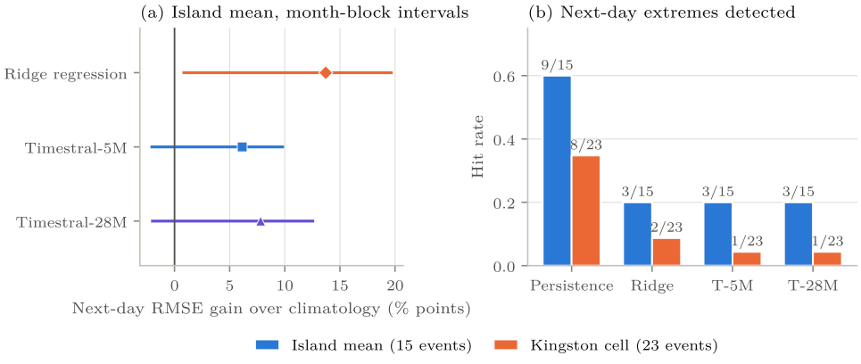
The month-block bootstrap estimate of Timestral-5M’s zero-delay island next-day RMSE gain over climatology is 6.14 % with interval percentage points; for the 28M it is 7.81 % with . Both cross zero, so on next-day RMSE neither checkpoint is distinguishable from climatology under this scheme. The 28M’s island seven-day change is −9.67 % with , worse than climatology under this scheme. The same analysis for ridge (Table 2) excludes zero at one day for both sites under zero delay and nowhere under the 45-day lag.
Timestral-5M’s 80 % nominal daily interval covers 84.3 % of island next-day outcomes and 88.1 % at Kingston under zero delay. Coverage exceeds the nominal rate by four to eight percentage points in these samples. The reference also carries observational error, and a calibrated seven-day interval would need a dependence-aware construction, since a sum of daily quantiles is not a quantile of the sum.
| Series, horizon | 0-d gain | 0-d 95 % interval | 45-d gain | 45-d 95 % interval |
|---|---|---|---|---|
| Island, 1 d | 13.71 | [0.85, 19.66] | 0.45 | [2.88, 0.45] |
| Island, 3 d | 6.03 | [1.19, 13.97] | 0.48 | [2.00, 0.85] |
| Island, 7 d | 3.69 | [0.67, 8.11] | 0.84 | [3.44, 0.90] |
| Kingston, 1 d | 12.36 | [4.08, 14.88] | 0.18 | [3.00, 0.63] |
| Kingston, 3 d | 5.77 | [0.34, 12.01] | 0.86 | [3.38, 0.64] |
| Kingston, 7 d | 3.74 | [0.20, 7.68] | 1.28 | [4.23, 0.98] |
4.3 Stale observations
With a 45-day delay, climatology has the lowest RMSE of the six methods at every site and horizon. The two Timestral checkpoints have island next-day RMSE 8.28 mm and Kingston 6.24 to 6.25 mm, against 7.82 and 5.77 for climatology. Ridge’s gains turn small and negative, from about to percentage points. Because the archive is finalised this says nothing about what an operational 45-day product would score; what it shows is that stale history erases the archive-model advantage.
4.4 Extremes
In the zero-delay island series the fitting-period 95th percentile is about 14.17 mm and 15 weekly test origins exceed it. Persistence forecasts 17 exceedances and hits 9 (hit rate 0.60, with 8 false alarms); ridge forecasts 4 and hits 3; each Timestral size detects 3 (hit rate 0.20). At Kingston the threshold is about 9.57 mm with 23 observed extremes; persistence forecasts 12 and hits 8, ridge forecasts 3 and hits 2, and each Timestral size detects 1. Ridge’s continuous RMSE advantage coexists with poor detection of rare heavy days, and neither pretrained model should be used for local extreme-rainfall alerts on this evidence. The counts are small and CHIRPS aggregation suppresses localised storms.
5 Computational checks
Three levels of checking were run. Data auditing confirms consecutive dates, non-negative finite values and checksums. An independent verifier reconstructs every unique target from the raw daily file, checks the score arithmetic and perturbs observations after issue time to confirm that earlier feature vectors do not change; all 1,872 unique scored windows were recomputed. A pinned claim-recount script then compared 192 numerical claims (sample size, RMSE, MAE and bias for 48 classical forecast groups) with an independent recount; all 192 matched at their reporting precision and a deliberately planted wrong count failed with exactly one finding. What these checks cover is numerical reproducibility and causal feature construction; the representativeness of CHIRPS, product availability, storm severity and the models’ pretraining data lie outside them.
6 Discussion
A locally fitted linear model uses short-memory structure in the archive, and that advantage is fragile, because a strict as-issued analysis needs provisional product versions and timestamps or a source with comparable near-real-time availability. Model size and public rank do not guarantee local extreme skill; both checkpoints improve typical next-day error and miss most heavy days. Timestral’s useful properties, a multivariate interface, known-future covariates and quantiles, are capabilities still to be tested with aligned inputs and proper scores; they are not demonstrated Jamaican gains.
A physics-informed extension would need a defined physical quantity. Surface precipitation is a flux from moisture transport and microphysics, not a conserved scalar in a two-dimensional rain field. The natural starting point is the vertically integrated moisture balance , which needs atmospherically consistent inputs and cannot be tested on two rainfall series. Any such model has to beat the baselines established here on the same dates.
Forecast value has several dimensions [9]. Agricultural users need weekly totals, flood officers need short-lead extremes and false-alarm rates, planners need return periods. A Caribbean trial should therefore involve the Meteorological Service of Jamaica, verified gauges and decision-sensitive scores, since low-resolution RMSE tells none of those users what they need to know.
7 Limitations and next experiments
The reference is a blended satellite-station estimate, not gauge truth, and the island mean and one cell hide finer variability. Weekly origins yield only 15 and 23 one-day extremes. The 45-day delay is a stress test on a finalised archive, and no numerical weather prediction was compared. The checkpoints ran at default zero-shot settings with a fixed context and no covariates, fine-tuning or recalibration. On the model side the checkpoint revision is unpinned and pretraining overlap with CHIRPS is unknown. The 209M model is untested.
The prespecified primary follow-up is zero-shot Timestral-209M against the same controls on the same 312 origins, with next-day RMSE gain over climatology under zero delay as the primary endpoint and the 45-day comparison as the stress test. Further experiments should compare Timestral with TimesFM and Chronos under identical normalisation, missingness, dates and horizons; use quality-controlled gauges, as-issued weather forecasts and versioned near-real-time satellite inputs; extend to several physiographic regimes and watersheds; and test moisture-budget constraints against matched non-physics controls.
8 Conclusion
On the fixed Jamaican dataset, both zero-shot Timestral checkpoints have lower next-day MAE than the four local controls. Neither has the lowest RMSE. Persistence has lower RMSE at one day, and ridge regression at three and seven days. At the island mean, the longer-horizon ridge advantage is about 10 to 12 %. Their island-mean next-day month-block intervals for RMSE gain over climatology cross zero, whereas ridge’s next-day interval does not; they detect three of fifteen island-mean extremes against persistence’s nine; and under a 45-day observation delay climatology has the lowest RMSE at every tested site and horizon. The findings fix the local baselines that any foundation or physics-informed model has to beat on these dates. They say nothing about operational skill, which needs as-issued inputs and gauge verification.
Data and code availability
CHIRPS v2 is public and the two-series file is identified by its SHA-256 above. The run package (acquisition and feature code, the ridge selections, the Timestral forecast arrays, the 1,872 scored windows, the bootstrap draws and the recount logs) is held in the author’s archive and is available on request. Timestral checkpoints are distributed by Mistral under their own licence.
References
[1] Abhimanyu Das, Weihao Kong, Rajat Sen, and Yichen Zhou. A decoder-only foundation model for time-series forecasting. In Proceedings of the 41st International Conference on Machine Learning (ICML), 2024. arXiv:2310.10688.
[2] Abdul Fatir Ansari, Lorenzo Stella, Caner Turkmen, Xiyuan Zhang, Pedro Mercado, Huibin Shen, Oleksandr Shchur, Syama Sundar Rangapuram, Sebastian Pineda Arango, Shubham Kapoor, Jasper Zschiegner, Danielle C. Maddix, Hao Wang, Michael W. Mahoney, Kari Torkkola, Andrew Gordon Wilson, Michael Bohlke-Schneider, and Yuyang Wang. Chronos: Learning the language of time series. arXiv:2403.07815, 2024.
[3] Mistral AI. Introducing Timestral. https://mistral.ai/news/timestral/, 2026. 15 October 2026.
[4] Mistral AI. Timestral: official inference code, documentation, model sizes and licensing. https://github.com/mistralai/timestral, 2026. Accessed 16 October 2026; checkpoint revision not pinned in the v0.2 run.
[5] Puja Das, August Posch, Nathan Barber, Michael Hicks, Kate Duffy, Thomas Vandal, Debjani Singh, Katie van Werkhoven, and Auroop R. Ganguly. Hybrid physics-AI outperforms numerical weather prediction for extreme precipitation nowcasting. npj Climate and Atmospheric Science, 7: 282, 2024. doi: 10.1038/s41612-024-00834-8.
[6] Suman Ravuri, Karel Lenc, Matthew Willson, Dmitry Kangin, Remi Lam, Piotr Mirowski, Megan Fitzsimons, Maria Athanassiadou, Sheleem Kashem, Sam Madge, Rachel Prudden, Amol Mandhane, Aidan Clark, Andrew Brock, Karen Simonyan, Raia Hadsell, Niall Robinson, Ellen Clancy, Alberto Arribas, and Shakir Mohamed. Skilful precipitation nowcasting using deep generative models of radar. Nature, 597: 672–677, 2021. doi: 10.1038/s41586-021-03854-z.
[7] Chris Funk, Pete Peterson, Martin Landsfeld, Diego Pedreros, James Verdin, Shraddhanand Shukla, Gregory Husak, James Rowland, Laura Harrison, Andrew Hoell, and Joel Michaelsen. The climate hazards infrared precipitation with stations: a new environmental record for monitoring extremes. Scientific Data, 2: 150066, 2015. doi: 10.1038/sdata.2015.66.
[8] Climate Hazards Center. CHIRPS2 FAQ: spatial resolution, time steps, units and product latency. https://wiki.chc.ucsb.edu/CHIRPS2_FAQ, 2026. Accessed 16 October 2026.
[9] Allan H. Murphy. What is a good forecast? An essay on the nature of goodness in weather forecasting. Weather and Forecasting, 8 (2): 281–293, 1993. doi: 10.1175/1520-0434(1993)008<0281:WIAGFA>2.0.CO;2.