Keywords: CHIRPS; Caribbean; daily rainfall; data latency; calibration; isotonic regression; transfer; regional pooling; Brier score.
1 Introduction
A rainfall model evaluated against a final historical product sees the most recent values available. An operational forecast may not have those finalised values at issue time. This paper tests a fixed small neural regressor and classifier against ridge regression, local logistic regression, persistence and seasonal climatology under three constraints that an operational Caribbean system would face: the newest rainfall input is days or weeks old; probabilities must be credible on later data, not on the period used to fit a calibration map; and a target location has only a year or three of labels. The question is under which of these constraints a small deep model is worth preferring to a well-regularised linear one.
The three experiments share one archive, one feature set, one network and one evaluation protocol, so their results can be read together. None of them trains a physics-informed architecture. Their value is diagnostic. They establish which comparators, and which information sets, any later model has to beat.
2 Shared data, features and models
2.1 Archive and supports
Daily CHIRPS v2 rainfall [1] from 1 January 2010 to 31 December 2025 (5,844 values per series) was assembled for eight supports: an archived Jamaica grid mean and seven grid-cell requests through the public ClimateSERV API (datatype 0, daily interval, mean operation) at Kingston, eastern and western Jamaica, and single cells in Haiti, the Dominican Republic, Puerto Rico and Trinidad (Table 1). Request geometries, raw responses and hashes are retained. These are estimates on spatial supports rather than station observations, and a country name labels a convenience cell rather than a national sample. Calendar dates were checked against API epoch times, and the series contain no missing or negative values.
| Series | Longitude | Latitude | Support |
|---|---|---|---|
| Jamaica mean | 77.3000 | 18.1000 | area mean |
| Kingston | 76.7750 | 18.0250 | grid cell |
| East Jamaica | 76.3750 | 18.0750 | grid cell |
| West Jamaica | 77.9250 | 18.4250 | grid cell |
| Haiti cell | 72.3250 | 18.5750 | grid cell |
| Dominican cell | 69.9250 | 18.4750 | grid cell |
| Puerto Rico cell | 66.0750 | 18.4250 | grid cell |
| Trinidad cell | 61.4250 | 10.6250 | grid cell |
2.2 Features
Each row has 25 inputs: seven log-transformed rainfall lags (1, 2, 3, 5, 7, 14 and 28 days); log-transformed antecedent means and wet-day fractions over 3, 7, 14, 30 and 90 days; three annual sine-cosine harmonic pairs; and longitude and latitude. A wet day is at least 1 mm. Rolling features are computed after shifting the series by one day plus any assumed additional delay, so no target-day value and no centred window enters a feature. Rows with incomplete initial history are dropped. A future-perturbation check alters later rainfall values and confirms that earlier feature rows are unchanged.
2.3 Models and training
The network has two ReLU hidden layers of widths 32 and 16 and one output, 1,377 parameters. Inputs are standardised on training data only. For amounts the target is divided by its training standard deviation (minimum scale one), the loss is mean squared error and negative predictions are clipped to zero at inference; for occurrence the loss is binary cross-entropy with logits and a sigmoid is applied at inference. Adam runs at learning rate with weight decay for 80 epochs on shuffled minibatches of about 256 rows. Seeds 11, 29 and 47 are retained and averaged at prediction time, with CPU-deterministic algorithms.
Amount baselines are ridge regression with penalty 100 and non-negative clipping, a calendar-month mean from the applicable training labels, and persistence at the newest allowed observation. The occurrence baselines are local logistic regression with and the monthly event frequency. None of these choices was selected on 2022–2025 scores. Fits are static. Parameters are not updated through the test period, although recent observations from earlier test days may enter later test features, which the stated sequential information set permits.
2.4 Evaluation and uncertainty
Testing covers 1 January 2022 to 31 December 2025, 1,461 dates per support and model. Amounts are scored by RMSE, MAE and bias in mm/day; occurrence by Brier score, with log loss (probabilities clipped to ), AUC, probability bias and reliability bins as secondary diagnostics. Model differences are paired on identical dates and resampled with a circular moving-block bootstrap at 30- and 90-day blocks, 2,000 replicates and a fixed seed; 90-day percentile intervals are reported. They are conditional on the fitted models and the archive, uncorrected for the many site-model comparisons, and exclude observational uncertainty. Cells are never treated as independent replicates to manufacture narrow regional intervals [2]. Scalar primary scores and sample counts were recomputed independently from the saved prediction CSVs.
3 Experiment 1: stale inputs
3.1 Design
Two supports are evaluated separately, the Jamaica grid mean and the Kingston cell; a spatial average and a local cell are different targets and their errors are not a ranking of difficulty. For target day and assumed delay days, the newest rainfall predictor is . Zero delay still uses the preceding day’s total. The delayed scenario also shortens the training-label cut-off by days relative to 1 January 2018, which restricts labels conservatively at the nominal origin and introduces a small training-sample difference between delays that a controlled follow-up should separate. Delays are analyst-defined scenarios; verified CHIRPS release times would be the operational version of the test.
3.2 Result
The network’s advantage over climatology is absent at seven days of added delay (Table 2). At zero added delay its Jamaica-mean RMSE is 6.871 mm/day against 7.598 for climatology, a 9.56 % reduction, with paired neural-minus-seasonal difference and 90-day interval . At 45 days the neural RMSE is 8.0145 against 7.6141 for climatology and the difference is with interval . Ridge is 6.9525 at zero delay and 7.6063 at 45 days; it degrades less than the network at every delay and is better than it from seven days on.
At Kingston with fresh inputs the neural RMSE is 4.510, ridge 4.393 and climatology 4.564 mm/day; the neural-minus-ridge difference is with interval , and the network’s small advantage over climatology does not exclude zero. So the zero-delay gain over climatology at the Jamaica mean cannot be attributed to non-linear modelling. A regularised linear combination of the same history and seasonal features extracts most of it, and does so more reliably when inputs are stale.
| Support | Delay (days) | Neural | Ridge | Seasonal |
|---|---|---|---|---|
| Jamaica mean | 0 | 6.8713 | 6.9525 | 7.5978 |
| Jamaica mean | 7 | 7.6651 | 7.5432 | 7.5990 |
| Jamaica mean | 21 | 7.9139 | 7.6022 | 7.5967 |
| Jamaica mean | 45 | 8.0145 | 7.6063 | 7.6141 |
| Kingston | 0 | 4.5097 | 4.3931 | 4.5644 |
| Kingston | 7 | 4.6971 | 4.5546 | 4.5654 |
| Kingston | 21 | 4.7466 | 4.5625 | 4.5629 |
| Kingston | 45 | 4.7732 | 4.5906 | 4.5654 |
At longer delays the network can fit historical relationships that are weak or unstable later; reduced persistence, estimation variance and a shifting rainfall distribution can all contribute and the design does not separate them. A forecast labelled “one day ahead” must also state the date of its newest observation.
4 Experiment 2: recalibration tested on a later period
4.1 Design
The event is at the seven cells. A pooled network shares parameters across cells with coordinates as predictors, while logistic regressions are fitted per cell, so the neural-versus-logistic comparison mixes data sharing with model class. Models are trained before 2018. Isotonic regression is fitted separately for each site and model family on 2020–2021, with out-of-range inputs clipped to the fitted map, and its effect is scored only on 2022–2025. The 2018–2019 period is reserved and unused. The threshold was fixed before any score was inspected; it measures ordinary wet-day occurrence, and a hazard study would need thresholds of its own.
4.2 Result
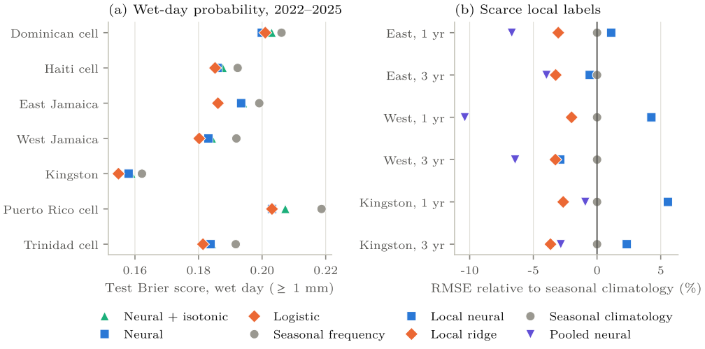
Isotonic recalibration raises the neural model’s Brier score at all seven cells. Raw local logistic regression has a lower Brier score than the raw pooled network at five of seven; at the Puerto Rico cell the two are equal at the printed precision and at the Dominican cell the network is better by 0.0011. For logistic regression the same map is close to neutral. It lowers the Brier score at three cells by at most 0.0005 and raises it at four by up to 0.0018. Equally weighted site means are 0.18454 for raw logistic, 0.18675 for raw neural, 0.18846 for recalibrated neural and 0.19457 for seasonal frequency (Table 3); these means are descriptive, and seven convenience cells do not stand for the Caribbean.
The per-site changes are small, and their intervals show why a consistent direction should not be reported as uniform certainty. At Kingston the recalibrated-minus-raw difference is with interval ; at the Dominican cell it is with . A visually close pooled reliability curve does not overturn the proper-score result, because coarse bins average over cases and a pooled curve can combine over-prediction at one cell with under-prediction at another.
| Cell | Neural + iso | Neural | Logistic + iso | Logistic | Seasonal |
|---|---|---|---|---|---|
| Dominican cell | 0.2030 | 0.1999 | 0.2005 | 0.2010 | 0.2061 |
| Haiti cell | 0.1876 | 0.1860 | 0.1870 | 0.1852 | 0.1923 |
| East Jamaica | 0.1940 | 0.1934 | 0.1866 | 0.1861 | 0.1991 |
| West Jamaica | 0.1842 | 0.1831 | 0.1800 | 0.1802 | 0.1919 |
| Kingston | 0.1589 | 0.1580 | 0.1565 | 0.1548 | 0.1622 |
| Puerto Rico cell | 0.2073 | 0.2031 | 0.2029 | 0.2031 | 0.2187 |
| Trinidad cell | 0.1843 | 0.1838 | 0.1823 | 0.1814 | 0.1917 |
A monotone map can correct systematic distortion, but its steps depend on the calibration sample, and when the map drifts or the original probabilities are already adequate for the sample size, recalibration adds estimation error. The experiment is consistent with that account and does not identify the mechanism. Calibration must be tested on a strictly later period, with an unrecalibrated comparator retained.
5 Experiment 3: scarce local labels and regional pooling
5.1 Design
The targets are the Kingston, western and eastern Jamaica cells. Local training labels are restricted to 2017 alone or to 2015–2017. The pooled fit adds 2010–2017 records from the six other cells, which include the other Jamaican cells, so a pooled gain cannot be attributed to cross-country transfer specifically. Local and pooled networks share architecture, optimiser, epochs and seeds. They do not share computation, since the pooled model sees many more examples and updates per epoch. Scarcity applies to training labels only; each target’s recent rainfall history remains available at test time, so the design says nothing about an unmonitored location. This is pooled supervised learning; zero-shot transfer is a different experiment.
5.2 Result
Pooled RMSE is lower than local neural RMSE in all six target-window configurations (Table 4). With one year of labels the local network is worse than seasonal climatology at all three cells, so the local fit is the weakest comparator in the table. With one year of labels, West Jamaica improves from 13.119 to 11.275 mm/day, a paired difference of with interval ; East Jamaica improves from 16.802 to 15.505, difference with interval . Local ridge is nonetheless better than pooling at Kingston: 4.532 against 4.612 with one year and 4.420 against 4.457 with three. At the eastern and western cells the pooled network beats local ridge in the point estimates for both windows, and the three-year intervals include zero.
| Target | Local years | Local neural | Local ridge | Seasonal | Pooled neural |
|---|---|---|---|---|---|
| East Jamaica | 1 | 16.8022 | 16.1117 | 16.6179 | 15.5053 |
| East Jamaica | 3 | 16.1242 | 15.6902 | 16.2169 | 15.5729 |
| West Jamaica | 1 | 13.1190 | 12.3304 | 12.5821 | 11.2754 |
| West Jamaica | 3 | 11.7694 | 11.7232 | 12.1195 | 11.3396 |
| Kingston | 1 | 4.9144 | 4.5317 | 4.6554 | 4.6124 |
| Kingston | 3 | 4.6947 | 4.4199 | 4.5876 | 4.4569 |
Kingston is the instructive case. Borrowing data improves on a local neural fit, and that is a weaker claim than beating the best local statistical method. If the local network estimates too many degrees of freedom from a short sample, pooling regularises it without creating an advantage over ridge. Three years of labels narrow the gap, but the experiment tests the specified years ending in 2017 and does not vary the training origin, so no sample-efficiency claim is made.
6 Discussion
Three features of the design limit what else can be said. All labels come from one gridded product, so a model can learn shared retrieval structure; independent gauge verification is needed before any gain is read as rainfall knowledge. The network is one fixed small architecture and the ridge penalty one fixed value, without tuning, so nothing here is a general statement about linear against non-linear models. Overlapping Jamaican years were examined in earlier work, which makes all three studies exploratory rather than prospective.
The next experiments follow from the gaps. For latency, retrieve versioned near-real-time inputs and compare forecasts issued on the same dates, with a numerical weather prediction baseline and gauge verification on decision-relevant accumulation windows. For calibration, run a factorial design with pooled logistic regression, local neural classifiers, regularised calibration and matched sample weighting, and add hazard thresholds fixed independently of the test outcomes. For pooling, hold out an entire island during model selection, admit controlled amounts of local data, match update budgets, and fit source-only, within-Jamaica-only and external-only models to find where the useful information originates. A terrain-aware model is the natural extension, and it has to be measured against the pooled baseline on the same data.
7 Conclusion
Read together, the three experiments give the entry conditions for a deep rainfall model in this setting. Fresh inputs come first, because the Jamaica-mean advantage over climatology is absent at seven days of added delay. A strong linear comparator belongs in every table. Ridge wins at Kingston with fresh inputs, degrades less with stale ones and beats pooled training at Kingston under label scarcity, and logistic regression beats the pooled classifier at five of seven cells. Calibration has to be tested out of period, since the isotonic map fitted on 2020–2021 worsened the neural Brier score at every tested cell in 2022–2025. With scarce local labels, pooled training improves the local neural model, but it does not outperform local ridge at every cell. All three studies are product-relative and exploratory, and none has independent gauge verification.
Data and code availability
The companion archive holds raw API responses, retrieval parameters, coordinates, merged data, feature and model code, neural checkpoints, predictions, complete score tables, uncertainty calculations and validation records. The original reports recounted every quoted claim from the prediction files with an independent script, with a deliberately altered claim as a negative control. The archive was not re-executed for this draft, so the numbers here are those of the archived reports rather than an independent replication.
References
[1] Chris Funk, Pete Peterson, Martin Landsfeld, Diego Pedreros, James Verdin, Shraddhanand Shukla, Gregory Husak, James Rowland, Laura Harrison, Andrew Hoell, and Joel Michaelsen. The climate hazards infrared precipitation with stations: a new environmental record for monitoring extremes. Scientific Data, 2: 150066, 2015. doi: 10.1038/sdata.2015.66.
[2] David R. Roberts, Volker Bahn, Simone Ciuti, Mark S. Boyce, Jane Elith, Gurutzeta Guillera-Arroita, Severin Hauenstein, José J. Lahoz-Monfort, Boris Schröder, Wilfried Thuiller, David I. Warton, Brendan A. Wintle, Florian Hartig, and Carsten F. Dormann. Cross-validation strategies for data with temporal, spatial, hierarchical, or phylogenetic structure. Ecography, 40 (8): 913–929, 2017. doi: 10.1111/ecog.02881.