Keywords: Jamaica; TimesFM; Chronos-2; satellite radiation; sea-surface temperature; physics-informed learning; temporal cross-validation; WeatherNext.
1 Introduction
Three claims are often bundled under the phrase “physics-informed forecasting”: that extra predictors help a learner, that exchange between neighbouring cells helps it use regional context, and that a physical penalty helps a network that already has those inputs. They need three different comparisons. The question here is whether any of the three additions (satellite and ocean predictors, exchange between neighbouring cells, a reduced physical penalty) improves seven-day temperature forecasts over a frozen foundation model and a traditional baseline. This paper runs all three comparisons on one target, daily mean two-metre temperature at three ERA5-derived cells labelled Kingston, Montego Bay and Mandeville, with seven-day forecasts issued every Monday.
The inputs are deliberately limited to what a small regional group can obtain and version. NASA POWER supplies daily radiation and cloud products; NOAA OISST supplies two offshore sea-surface temperature (SST) series; three further ERA5 cells supply air-temperature context. Frozen TimesFM 2.5, TimesFM 3 and Chronos-2 forecasts enter as predictors and as standalone comparators. A small graph network with a symmetric, bounded exchange term supplies local corrections; it has local neural cores and a conservative exchange between them, and I refer to it as the exchange graph network.
The contribution is an executed comparison that keeps the three questions apart. Matched ablations isolate the satellite feature package, the graph expansion and the physics penalty. A smoothness control tests whether a generic temporal penalty explains any gain from the physical one. A separate comparison scores actual WeatherNext 2 and ECMWF IFS archive outputs on their common dates, so their skill is measured and never inferred from a model card.
The evaluation periods require a qualification. This is the third study on these cells, and earlier rounds inspected the 2023–2025 evaluation years. Reusing a period does not make it an independent holdout [1], so this round is exploratory even though its search is bounded and its model choices were frozen before the outer scores were read.
2 Related work and baselines
Persistence, seasonal naive forecasting, exponential smoothing, autoregression and dynamic harmonic regression are the benchmarks a seasonal daily series should be judged against [2]. A complex model should improve on a reasonably fitted traditional alternative. A weak climatological baseline alone cannot establish that benefit. The principal traditional comparator is therefore an AR(14) model fitted to a trailing 1,095-day anomaly series. The wider set includes persistence, a 365-day seasonal naive forecast, simple exponential smoothing with coefficient 0.1, damped Holt smoothing, two-harmonic dynamic regression with a 1,825-day window and a regularised VAR(1).
TimesFM is a decoder-only foundation model for time series [3, 4, 5]; Chronos-2 is a separately pretrained family [6]. Their checkpoints remain fixed in this study. The local models learn forecast corrections rather than retrain the foundation models.
A physics-informed penalty punishes disagreement with a chosen equation [7]. It does not guarantee the equation is adequate for the target, and stronger enforcement can hurt [8]. Reported gains from hybrid physics-AI nowcasting of extreme precipitation [9] concern radar, convective scales and a different variable, so they motivate the test here and transfer no evidence to daily temperature at three grid cells.
3 Data and admissible information
3.1 Targets and context cells
Daily records from 1 January 2010 to 30 September 2026 (6,117 days) were retrieved for six cells through the Open-Meteo historical API with the ERA5 model specified, nearest-cell selection and the America/Jamaica time zone [10, 11, 12]. Elevation adjustment was disabled. The target is the returned gridded product and no quality-controlled station enters. Place names identify requested locations, and the returned cells smooth the terrain; the Mandeville-labelled cell (model elevation 265 m) does not resolve the town’s highland microclimate. Table 1 lists the cells.
| Cell label | Lat. (°N) | Lon. (°E) | Elevation (m) | Role |
|---|---|---|---|---|
| Kingston | 18.00 | 76.75 | 246 | Target |
| Montego Bay | 18.50 | 78.00 | 130 | Target |
| Mandeville | 18.00 | 77.50 | 265 | Target |
| Port Antonio | 18.25 | 76.50 | 0 | Context |
| May Pen | 18.00 | 77.25 | 280 | Context |
| Savanna-la-Mar | 18.25 | 78.25 | 0 | Context |
Two of the three context cells return zero elevation and so sample coastal rather than inland conditions, which makes their inclusion a mixed intervention on regional context rather than a clean test of ocean influence.
3.2 Satellite-derived products
NASA POWER supplies daily all-sky and clear-sky downward shortwave radiation and cloud amount; the retrieved headers identify CERES SYN1deg as the source [13]. The native solar grid is about one degree, coarser than the target grid, and the six requests return only three distinct radiation histories: Kingston shares a series with Port Antonio, and Mandeville, May Pen and Montego Bay share another. That duplication is retained and documented; nothing here presents six independent observations. All-sky radiation in kWh m−2 day−1 is converted to a daily mean in W m−2 by multiplying by ; the all-sky to clear-sky ratio is a further cloud feature.
NOAA OISST v2.1 supplies daily SST at 17.375 °N and 18.875 °N, both at 77.375 °W [14, 15]. OISST blends satellite and in-situ data through an analysis, so it is an analysed field and no raw radiometer measurement. No altimetry or sea-level predictor is used; the two points sample conditions south and north of the island.
The source audit found 61 missing tail days in every POWER parameter, from 1 August to 30 September 2026, and 21 missing dates in each OISST series after alignment with a longest gap of nine days. All gaps are filled forward from past values only; no later observation is used. Whether an input was contemporaneous or carried forward is recorded as a diagnostic stratum.
3.3 Origins, lags and the retrospective boundary
Forecast origins are local Mondays after that day’s record; the next seven daily means form the target window, retained only if it stays within the origin’s calendar year. Target windows do not overlap, though histories and weather regimes remain dependent across weeks. There are 550 weekly origins from 2016, of which 192 fall in 2023 to September 2026 and 38 in January to September 2026.
Temperature histories hold 512 observations through the origin. POWER predictors are lagged seven days and OISST predictors fourteen. These retrospective lags do not reconstruct when the products became available. Finalised CERES SYN1deg data can arrive well after seven days, and the low-latency FLASHFlux product is different. Finalised ERA5-derived temperature is also supplied at the origin. The experiment therefore measures extrapolation of a reanalysis target under an idealised information set. An operational claim would need as-issued inputs and independent station verification.
4 Model formulation
4.1 Seasonal reference and predictor vector
Two annual Fourier harmonics and an intercept are fitted to 2010–2015 observations. For air cell , let be its seasonal reference and its anomaly. A trailing 90-day anomaly mean adapts the reference at origin : (1) Radiation, cloud, ratio and SST anomalies use analogous initialisation-period fits. Every rolling statistic stops at the applicable observation or lag date.
The per-cell input has 77 entries: 26 temperature, ERA5-radiation and calendar features; 22 satellite-radiation, cloud and ratio features; eight offshore-SST features; and three seven-day forecast vectors expressed relative to . The forecast vectors are TimesFM 2.5, the original TimesFM 3 variant and a satellite/context TimesFM 3 variant at the three targets. At context cells, where no TimesFM inference was run, all three slots hold a past-only AR(14) forecast.
The satellite/context TimesFM 3 variant receives the three target series plus fourteen past-only covariates over 512 days: three ERA5-radiation histories, three context air-temperature histories, six radiation and cloud histories and the two SST histories. It changes several input groups at once, so its difference from the original variant is an input-bundle comparison. The narrower satellite test is the matched local-network ablation below.
4.2 Local cores and symmetric exchange
Each local core is a shared network with tanh hidden layers and a bounded output . With the last hidden state and an approximate horizontal distance in kilometres, (2) where is the logistic function. The conductance matrix is symmetric and non-negative with row sums at most 0.15. The exchange at lead is (3) so up to floating-point error. Because areas, heat capacities and boundary-layer depths are unresolved, this conserves the sum of model anomalies under equal implicit capacities and nothing more; it is an algebraic budget, and the atmospheric energy budget is a separate quantity.
With the base forecast anomaly (TimesFM 2.5 at targets, AR(14) at context cells, ), the corrected forecast is (4) Setting removes exchange. No supervised target is added at context cells. The primary-cell graph keeps edges only among the three targets; the six-cell graph keeps all edges.
4.3 Reduced closure and matched controls
A phenomenological daily closure supplies relaxation, radiation and ocean terms, (5) where extrapolates the last admissible satellite-radiation anomaly with an initialisation-fitted AR(1) decay and does the same for the mean of the two SST anomalies. Coefficients are fitted by bounded least squares on 2010–2015 transitions with and . The bounds stabilise fitting; they are not physical constants, and the coefficients absorb unit conversions. The closure omits advection, humidity, longwave radiation and turbulent fluxes, and it is fitted around the fixed seasonal reference but applied around the rolling one, which drops the mean-level source introduced by recentring. The term PINN here means a discrete, reduced-order physics-informed network rather than a continuous PDE solver, and the closure is the place where the two differ most.
With residual scale fitted during initialisation, the full penalty is (6) The Huber threshold is 0.2 °C. The physics term applies to all six cells; the data term to the three targets. Relaxation-only and relaxation-plus-radiation variants refit their own coefficients and scales. A smoothness control penalises with the full-closure scale, which tests whether a generic temporal penalty explains any gain.
All neural variants share width, depth, optimiser (AdamW, learning rate , weight decay ), 150 updates and seeds 11, 23 and 37, whose forecasts are averaged. The penalty weight is chosen from on the inner folds. The full PINN and its unpenalised graph counterpart share inputs, base forecasts, scaling, architecture and seeds; the penalty is the intended difference. The no-satellite network zeroes the satellite and ocean features and the satellite/context TimesFM block, so no satellite information leaks in through that forecast vector.
5 Selection, evaluation and uncertainty
5.1 Nested temporal selection with a finite budget
Inner validation years are 2020, 2021 and 2022; a model scored on a year is fitted only to earlier origin years. Outer models are refitted annually for 2023 to 2026 with the configuration choices carried over from the inner folds, so earlier outer years become training data for later refits. Feature standardisation is fitted inside each training set.
An 18-trial tree-structured Parzen estimator search [16, 17] selects among ridge, extra-trees and histogram gradient-boosting corrections, a three-, six- or ten-year training window and a TimesFM 2.5 or satellite/context TimesFM 3 anchor. The search totals 54 inner ML fits, 12 neural configurations with 108 seed-level inner fits, 96 seed-level annual outer fits and six stacking settings. Code and fitted choices were hashed before the outer results were summarised. The search stops at the fixed budget and does not use outer-test results to select further trials.
Two non-negative, unit-sum stacking ensembles combine five foundation and traditional forecasts, the selected ML correction and eight neural families, using out-of-fold 2020–2022 predictions. One ensemble is unrestricted; the other must give at least 10 % weight to the full PINN. The constraint tests the requested physics-containing combination; it does not make the physics contribution optimal. Table 2 lists the frozen choices.
| Choice | Selected setting |
|---|---|
| ML correction | Extra trees; 160 trees; depth 8; minimum leaf 18 |
| ML window / anchor | Ten years / satellite-context TimesFM 3 |
| Neural width / updates | 16, 16 / 150 |
| Seeds | 11, 23, 37 |
| Penalty weight | 0.1 for all four penalty families |
| Stacking shrinkage | 0 for both ensembles |
| Full-PINN weight | 3.72 % unrestricted; 10.00 % constrained |
5.2 Scores and paired intervals
MAE is averaged equally over the three targets, the weekly origins and the seven leads; RMSE and signed bias supplement it. Relative improvement is , always between named models on the same targets. Hot-day and rapid-change strata use each cell’s initialisation-period 90th percentile of temperature and 95th percentile of absolute daily change, fixed without reference to outer errors.
For paired uncertainty, absolute-error differences are averaged over sites and leads within each origin, and a circular moving-block bootstrap [18] resamples those origin clusters 10,000 times with two-, four- and eight-week blocks. Four-week intervals are the principal summary. They condition on the fitted models and the one observed sequence, and they say nothing about retraining, predictor selection or the reuse of inspected years. No stopping decision used these intervals, and an interval that excludes zero is reported as descriptive support rather than confirmatory significance.
5.3 WeatherNext and IFS archive comparison
Actual WeatherNext 2 ensemble-mean outputs and ECMWF IFS 0.25 ° outputs were retrieved through Open-Meteo’s previous-runs service with the same point requests and daily aggregation [19, 20]. Local WeatherNext weights were reviewed but not executed; the official inference path needs global multivariate inputs and accelerators the CPU-based experiments here did not have. The retrieved product is a fixed-lead archive: the forecast for target day is the field with nominal offset hours, and a daily mean is formed only when all 24 local hours are finite. The weekly vector is therefore not necessarily one coherent initialisation. Only dates with complete seven-day predictions for all three targets in both services enter the cohort, and every local model is rescored on exactly those dates. A prespecified 50:50 WeatherNext-ensemble blend is also scored, with no weight fitted on the cohort.
6 Results
6.1 The ensemble beats AR(14); TimesFM remains competitive
The PINN-constrained ensemble reaches a pooled MAE of 0.4966 °C over 2023 to September 2026 against 0.5167 °C for AR(14), a 3.89 % reduction. Its margin over TimesFM 2.5 is 0.0018 °C, or 0.35 %. The original TimesFM 3 variant has the lowest pooled MAE of any model, 0.4959 °C, so against the strongest foundation-model result the ensemble has no advantage on this period; it is 0.0007 °C worse.
In 2026 the ensemble’s MAE is 0.5017 °C against 0.5349 °C for AR(14), a 6.22 % reduction. Dynamic harmonic regression is the strongest traditional model on that subset at 0.5261 °C, a ranking that is descriptive because it was read after the fact. TimesFM 2.5 is better on MAE, 0.4947 °C, so the ensemble is 1.41 % worse by that score; it is 1.73 % better on RMSE (0.7548 against 0.7681 °C). Table 3 gives the full set and Table 4 the year-by-year picture.
| Model | 2023–26 MAE | 2026 MAE | 2026 RMSE | Skill vs AR(14) (%) |
|---|---|---|---|---|
| Persistence | 0.5921 | 0.6499 | 1.0484 | -21.49 |
| Seasonal naive | 0.8610 | 0.7254 | 1.0273 | -35.61 |
| SES () | 0.5264 | 0.5558 | 0.8131 | -3.91 |
| Damped Holt | 0.5734 | 0.6329 | 0.9247 | -18.31 |
| DHR (2 harmonics, 1825-day window) | 0.5334 | 0.5261 | 0.7819 | +1.65 |
| Regularised VAR(1) | 0.5388 | 0.5886 | 0.8297 | -10.04 |
| AR(14) anomaly model | 0.5167 | 0.5349 | 0.7793 | +0.00 |
| TimesFM 2.5 | 0.4984 | 0.4947 | 0.7681 | +7.52 |
| TimesFM 3 original | 0.4959 | 0.5025 | 0.7699 | +6.07 |
| TimesFM 3 satellite | 0.4984 | 0.5041 | 0.7695 | +5.77 |
| Chronos-2 | 0.4976 | 0.5161 | 0.8039 | +3.51 |
| ML correction (extra trees) | 0.5033 | 0.5157 | 0.7643 | +3.60 |
| Local NN, no satellite | 0.5010 | 0.5125 | 0.7546 | +4.19 |
| Local NN, satellite | 0.5187 | 0.5112 | 0.7523 | +4.43 |
| Graph NN, primary cells | 0.5206 | 0.5120 | 0.7525 | +4.29 |
| Graph NN, six cells | 0.5254 | 0.5258 | 0.7747 | +1.71 |
| Graph NN, smoothness penalty | 0.5230 | 0.5227 | 0.7691 | +2.28 |
| Graph PINN, relaxation | 0.5246 | 0.5278 | 0.7810 | +1.33 |
| Graph PINN, relaxation + radiation | 0.5242 | 0.5249 | 0.7792 | +1.87 |
| Graph PINN, full closure | 0.5195 | 0.5142 | 0.7642 | +3.87 |
| Unrestricted ensemble | 0.4978 | 0.5041 | 0.7556 | +5.77 |
| PINN-constrained ensemble | 0.4966 | 0.5017 | 0.7548 | +6.22 |
| Model | 2023 | 2024 | 2025 | 2026 |
|---|---|---|---|---|
| AR(14) anomaly model | 0.5739 | 0.5607 | 0.4011 | 0.5349 |
| TimesFM 2.5 | 0.5378 | 0.5329 | 0.4265 | 0.4947 |
| TimesFM 3 original | 0.5366 | 0.5306 | 0.4148 | 0.5025 |
| Graph NN, six cells | 0.5657 | 0.5817 | 0.4275 | 0.5258 |
| Graph PINN, full closure | 0.5553 | 0.5856 | 0.4204 | 0.5142 |
| PINN-constrained ensemble | 0.5365 | 0.5420 | 0.4068 | 0.5017 |
6.2 Closure comparisons in 2026 and across the full period
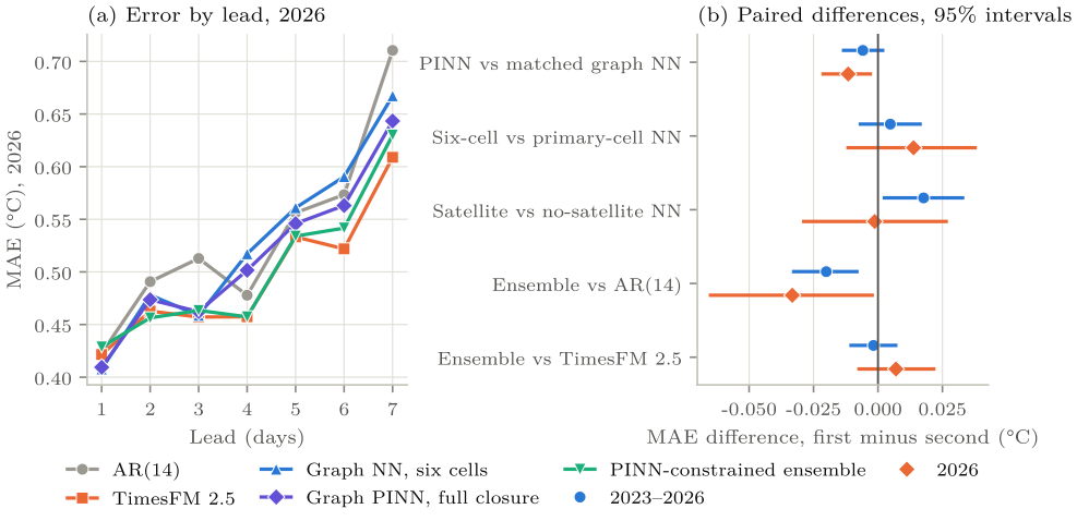
The full PINN has a 2026 MAE of 0.5142 °C against 0.5258 °C for the same graph network trained without the penalty. The 2.20 % reduction is a paired difference of −0.0116 °C with four-week interval ; the two- and eight-week intervals also exclude zero, and each of the three seeds improves under the penalty. Across all 192 origins the matched difference is −0.0059 °C with interval . The penalty helps in 2023, 2025 and 2026 and hurts in 2024 (Table 4). The evidence supports a benefit for this architecture in the 2026 subset.
Relaxation alone gives a 2026 MAE of 0.5278 °C; adding radiation gives 0.5249; the full closure with SST gives 0.5142; the smoothness control gives 0.5227 °C. The full closure is 1.63 % better than the smoothness control and 2.04 % better than the radiation-only closure. Because each variant refits its own coefficients and scales, these are comparisons between complete penalty families rather than isolated coefficient interventions. The full-closure residual RMS falls from 0.2746 in the unpenalised network to 0.2304 under the full penalty, a 16.10 % decrease, but the smoothness penalty also lowers it, to 0.2374 (Table 5). Closer agreement with the reduced equation is partly obtainable from generic regularisation; the extra predictive gain in 2026 is the evidence that the closure does something more, and it has to be weighed against the weak full-period result.
| Matched graph architecture | 2026 MAE | Full-closure residual RMS | Max |
|---|---|---|---|
| Graph NN, six cells | 0.5258 | 0.2746 | 5.6e-09 |
| Graph NN, smoothness penalty | 0.5227 | 0.2374 | 7.5e-09 |
| Graph PINN, relaxation | 0.5278 | 0.2468 | 7.5e-09 |
| Graph PINN, relaxation + radiation | 0.5249 | 0.2469 | 5.6e-09 |
| Graph PINN, full closure | 0.5142 | 0.2304 | 5.6e-09 |
6.3 Satellite predictors and extra cells do not reliably help
For the matched local networks, the satellite and ocean feature package raises pooled MAE from 0.5010 to 0.5187 °C, a 3.53 % increase with interval . In 2026 alone it lowers error slightly, from 0.5125 to 0.5112 °C, with an interval that spans both signs. The satellite/context TimesFM 3 variant is likewise a small degradation on the original, with pooled MAE 0.4984 against 0.4959 °C and 0.5041 against 0.5025 in 2026. The added predictors do not improve pooled error in these comparisons.
Adding the three context cells to the primary-cell graph raises 2026 MAE from 0.5120 to 0.5258 °C; the paired interval is wide, but the point estimate does not support the extra exchanges. Learned conductances are symmetric, obey the bounds and give a net exchange within of zero (Table 5). Those properties show what the implementation enforces, not that the links represent atmospheric transport. Table 6 collects the paired comparisons.
| Period | Paired comparison | Difference | 95% interval |
|---|---|---|---|
| 2023–2026 | Full PINN matched graph NN | -0.0059 | [-0.0133, +0.0018] |
| 2023–2026 | Six-cell primary-cell graph NN | +0.0048 | [-0.0068, +0.0163] |
| 2023–2026 | Satellite no-satellite local NN | +0.0177 | [+0.0025, +0.0328] |
| 2023–2026 | PINN ensemble AR(14) | -0.0201 | [-0.0327, -0.0082] |
| 2023–2026 | PINN ensemble TimesFM 2.5 | -0.0018 | [-0.0104, +0.0069] |
| 2026 | Full PINN matched graph NN | -0.0116 | [-0.0213, -0.0030] |
| 2026 | Six-cell primary-cell graph NN | +0.0138 | [-0.0116, +0.0377] |
| 2026 | Satellite no-satellite local NN | -0.0013 | [-0.0288, +0.0265] |
| 2026 | PINN ensemble AR(14) | -0.0333 | [-0.0650, -0.0023] |
| 2026 | PINN ensemble TimesFM 2.5 | +0.0070 | [-0.0074, +0.0216] |
The selected ML correction, an extra-trees model anchored on the satellite/context TimesFM 3 forecast, has a 2026 MAE of 0.5157 °C, worse than its 0.5041 °C anchor, yet it receives 42.39 % of the constrained ensemble’s weight. The other non-zero weights are 8.60 % TimesFM 2.5, 17.94 % original TimesFM 3, 21.07 % AR(14) and the required 10.00 % full PINN; the unrestricted ensemble gives the full PINN 3.72 %. Inner-fold stacking weights need not track later standalone rankings, and a non-zero physics weight is not evidence that the constraint is responsible for the ensemble’s skill.
6.4 Where the forecasts deteriorate
In 2026 the ensemble’s MAE rises from 0.4287 °C at lead one to 0.6300 °C at lead seven, a 46.95 % increase; the full PINN rises from 0.4094 to 0.6434 °C, 57.15 %. The full PINN’s lead-one error is below TimesFM’s 0.4215, and TimesFM has lower error at every later lead. The deterioration is steepest at days five to seven. By site, the ensemble’s 2026 MAE is 0.4017 at the Kingston cell, 0.5021 at Montego Bay and 0.6012 at Mandeville (Table 7); the inland cell is hardest for every model. Hot days are underpredicted and rapid cooling is missed, which is what one expects from a model that extrapolates recent local conditions with decayed forcing and no dynamical forecast of approaching circulation changes.
| Model | Kingston cell | Montego Bay cell | Mandeville cell |
|---|---|---|---|
| TimesFM 2.5 | 0.3891 | 0.5087 | 0.5863 |
| Graph PINN, full closure | 0.4265 | 0.5075 | 0.6086 |
| PINN-constrained ensemble | 0.4017 | 0.5021 | 0.6012 |
6.5 WeatherNext and IFS: raw errors are site offsets
The common cohort holds 16 weekly origins from 8 June to 21 September 2026, 336 site-lead targets. WeatherNext 2 has raw MAE 1.9172 °C and bias −1.8031 °C; IFS has MAE 2.5281 °C and bias −2.5034 °C (Table 8). WeatherNext’s raw MAE is 24.17 % lower than IFS on this comparison, but site offsets dominate this comparison and limit any conclusion about the two forecast systems. At the Montego Bay cell the two products have MAE 0.4578 and 0.4850 °C; at the Mandeville cell they have 4.4884 and 4.8757 °C, with every retained prediction colder than the target. Returned elevation metadata are 577 m for both services against 265 m for the ERA5 cell. Elevation points to a representativeness problem; how much of the offset it explains is still to be measured.
| Model or product | MAE | RMSE | Bias |
|---|---|---|---|
| AR(14) anomaly model | 0.4616 | 0.5767 | -0.3030 |
| TimesFM 2.5 | 0.3822 | 0.4936 | -0.1057 |
| PINN-constrained ensemble | 0.4081 | 0.5153 | -0.1855 |
| WeatherNext 2 archive (raw) | 1.9172 | 2.6927 | -1.8031 |
| ECMWF IFS archive (raw) | 2.5281 | 3.1566 | -2.5034 |
| WeatherNext + PINN ensemble (50:50) | 1.0781 | 1.4688 | -0.9943 |
After inspecting the raw comparison I added one bounded diagnostic. For each site and service, an additive mean-error offset was estimated from the first eight common origins (8 June to 27 July) and the last eight (3 August to 21 September, 168 targets) were scored. No lead-specific correction or blend weight was fitted. WeatherNext’s MAE falls from 2.0128 to 0.6077 °C on the scoring weeks, a 69.81 % reduction; IFS falls from 2.6544 to 0.5461 °C, 79.43 %, which reverses their raw ranking. The calibrated WeatherNext-ensemble blend has MAE 0.4868 °C, worse than the local ensemble’s 0.4389 and TimesFM’s 0.4120 °C (Table 9). Because the raw outcomes had been seen before the split was chosen, this remains a post hoc exploratory analysis.
| Model or product | MAE | RMSE | Bias |
|---|---|---|---|
| AR(14) anomaly model | 0.5247 | 0.6387 | -0.3274 |
| TimesFM 2.5 | 0.4120 | 0.5446 | -0.0672 |
| PINN-constrained ensemble | 0.4389 | 0.5593 | -0.1412 |
| WeatherNext 2 (raw) | 2.0128 | 2.7797 | -1.9581 |
| WeatherNext 2 (offset removed) | 0.6077 | 0.7865 | -0.3100 |
| ECMWF IFS (raw) | 2.6544 | 3.2681 | -2.6173 |
| ECMWF IFS (offset removed) | 0.5461 | 0.6964 | -0.2279 |
| Calibrated WeatherNext + PINN ensemble (50:50) | 0.4868 | 0.5892 | -0.2256 |
6.6 Comparison with the earlier rounds
On the same 798 targets in 2026 the previous round’s ensemble had MAE 0.5053 °C; the present ensemble has 0.5017, a 0.72 % reduction. Over the full 2023–2026 cohort the previous ensemble had 0.4965 and the present one 0.4966, the same score to three decimals. The new inputs and ablations improve understanding of the model’s behaviour more than they improve the best earlier pooled score. [earlier-round scores are taken from the previous manuscript archive and were not re-run]
7 Discussion
7.1 What improved and what did not
The ensemble lowers 2026 MAE by 6.22 %, 0.0333 °C in absolute terms, and its block-bootstrap interval favours it at every tested block length. TimesFM 2.5 alone lowers AR(14) error by 7.52 % on the same targets, which is why TimesFM stays the reference and the ensemble stays a research result.
Of the three ablations, the matched physics comparison is the most favourable. The full penalty improves the 2026 graph network for all three seeds, lowers the closure residual and beats the smoothness control, so the closure does more on that subset than impose generic smoothness. The pooled interval includes zero and the effect reverses in 2024. The defensible inference is that the reduced prior can stabilise this particular correction under some conditions.
The satellite ablation and the expanded TimesFM input show no consistent gain. Coarse duplicated pixels, strong predictor correlation, few supervised examples, stale tail observations and approximate lags are all plausible causes, and the design does not separate them. A feature can carry large conditional importance for a fitted network while the network generalises worse with it, which is what the permutation diagnostics and the matched ablation show together.
Context cells fail to show a reliable benefit either. The exchange is symmetric and distance-based; atmospheric transport is directional and regime-dependent. Symmetry enforces an exact anomaly budget but may suppress relevant directional contrasts. Context cells are unsupervised in the data loss and two of them are coastal zero-elevation cells.
7.2 Why performance falls away
Later-lead deterioration and missed rapid cooling are what a model does when it extrapolates recent local conditions without information about approaching circulation changes. Radiation and SST forcing are decayed from delayed observations, with no dynamical forecast to supply them, and a reduced equation cannot recover a missing driver. Hot-day underprediction indicates that shrinkage toward a learned reference improves typical errors while damping extremes.
WeatherNext and IFS add a dynamical source, but their point products do not match the ERA5 target domain, and the Mandeville offset plus the reversal after calibration show that representativeness has to be settled before a global-model ranking means anything. Removing an estimated offset does not establish which product is closer to the truth in the named settlements; that needs quality-controlled station data and consistent grid and height processing.
7.3 Limits on statistical and operational claims
The target is a third-party reanalysis product at three cells, not an observational network, and six correlated cells with two ocean samples do not resolve Jamaica’s terrain. Foundation-model pretraining overlap is unaudited. Earlier rounds inspected the evaluation years. Imposed lags do not reconstruct publication times, and finalised reanalysis is supplied at the origin. The archive cohort has sixteen complete origins under a fixed-lead convention, and its calibration diagnostic has eight scoring origins chosen after the raw results were seen. The intervals quantify variation in the retained paired losses conditional on the fitted models and the one historical sequence; they omit retraining, predictor selection, architecture search and the approximations in the closure. None of the findings should be described as statistically established superiority, operational readiness or state-of-the-art forecasting. No experiment was dropped for failing to help the preferred model, and no outer score triggered another round of optimisation.
8 Next experiment and decision rule
The next study should first fix the observation and issuance pipeline: quality-controlled station daily temperature with documented elevation and exposure, consistent collocation of every forecast, retained raw fields and a versioned issue-time inventory, and either genuine low-latency radiation products or an explicit forecast of their unavailable values. Data age and missingness should be predictors, compared with the present carry-forward policy under a prespecified outage experiment.
Second, strengthen the physical inputs before growing the network. Add forecast wind, humidity, pressure, net radiation and surface-flux terms where available; test directional advection against the symmetric exchange; fit and validate the closure around the same evolving reference used in prediction or keep the recentring source term; and estimate capacity or area weights before calling the anomaly exchange an energy budget. A matched control should change one physical term at a time with everything else fixed.
Third, reserve a post-freeze period and more stations, freeze a small candidate set (AR(14), the strongest traditional alternative chosen within training, TimesFM 2.5, the compact full PINN and a bias-calibrated WeatherNext combination), agree a minimum useful improvement with the supervisors in advance, and size the study from the observed origin-level error dependence rather than from site-lead counts. If the interval is still too wide, collect more observations; searching until a threshold is crossed is the thing to avoid.
On the present evidence, TimesFM 2.5 is the reference for the next local forecasting trial. The PINN is a research component with a measurable matched-network benefit in 2026. Satellite augmentation, larger spatial coupling and WeatherNext blending remain hypotheses until they improve on that reference under new data.
9 Conclusion
At three Jamaican ERA5-derived cells a frozen TimesFM 2.5 forecast remains the reference for seven-day temperature. The constrained ensemble lowers MAE relative to AR(14) by 3.89 % over 2023 to 2026 and 6.22 % in 2026. Its small pooled MAE advantage over TimesFM 2.5 is uncertain, and its 2026 MAE is higher. Of the three additions tested, only the reduced physical closure shows a gain, and only inside its matched graph network in 2026 (2.20 %, with an interval that excludes zero; the full-period interval includes it). Satellite and ocean predictors raise the matched network’s pooled error by 3.53 %, context cells do not help, and the raw archive forecasts are dominated by site offsets. The findings support a modest gain over a traditional baseline and a conditional gain from the reduced prior; they do not support replacing a foundation model with a physics-augmented one.
Data and code availability
The evidence package (freeze SHA-256 1b4a78690cb5…41b0) holds the metrics table (4,320 rows), the bootstrap, regime, physics-diagnostic and calibrated-weather tables, the calibration offsets and a source audit. An independent recount of all primary MAE and RMSE rows from the archived predictions passed (3,520 rows). Checkpoint revisions for TimesFM 2.5, TimesFM 3 and Chronos-2 are pinned in the references. No foundation checkpoint was retrained, and the experiments ran on CPU. ERA5 through Open-Meteo, NASA POWER and NOAA OISST are public; the evidence package is held by the author and is available on request.
References
[1] Gavin C. Cawley and Nicola L. C. Talbot. On over-fitting in model selection and subsequent selection bias in performance evaluation. Journal of Machine Learning Research, 11: 2079–2107, 2010.
[2] Rob J. Hyndman and George Athanasopoulos. Forecasting: Principles and Practice. OTexts, Melbourne, 3rd edition, 2021. https://otexts.com/fpp3/.
[3] Abhimanyu Das, Weihao Kong, Rajat Sen, and Yichen Zhou. A decoder-only foundation model for time-series forecasting. In Proceedings of the 41st International Conference on Machine Learning (ICML), 2024. arXiv:2310.10688.
[4] Google Research. TimesFM 2.5 (200m, pytorch): model card and software. https://huggingface.co/google/timesfm-2.5-200m-pytorch; https://github.com/google-research/timesfm, 2026. Accessed 13 October 2026; checkpoint revision recorded in the provenance file.
[5] Google Research. TimesFM 3 model card and official implementation. https://huggingface.co/google/timesfm-3.0-pytorch, 2026. Accessed 14 October 2026; pinned weight revision 43046b85ec22d584a13f8098c2ed39c889e129c2.
[6] Amazon Science. Chronos-2: From univariate to universal forecasting. arXiv:2510.15821; https://huggingface.co/amazon/chronos-2, 2025. Accessed 14 October 2026; pinned revision 29ec3766d36d6f73f0696f85560a422f50e8498c.
[7] Maziar Raissi, Paris Perdikaris, and George Em Karniadakis. Physics-informed neural networks: A deep learning framework for solving forward and inverse problems involving nonlinear partial differential equations. Journal of Computational Physics, 378: 686–707, 2019. doi: 10.1016/j.jcp.2018.10.045.
[8] Aditi S. Krishnapriyan, Amir Gholami, Shandian Zhe, Robert M. Kirby, and Michael W. Mahoney. Characterizing possible failure modes in physics-informed neural networks. In Advances in Neural Information Processing Systems 34 (NeurIPS), 2021. arXiv:2109.01050.
[9] Puja Das, August Posch, Nathan Barber, Michael Hicks, Kate Duffy, Thomas Vandal, Debjani Singh, Katie van Werkhoven, and Auroop R. Ganguly. Hybrid physics-AI outperforms numerical weather prediction for extreme precipitation nowcasting. npj Climate and Atmospheric Science, 7: 282, 2024. doi: 10.1038/s41612-024-00834-8.
[10] Hans Hersbach, Bill Bell, Paul Berrisford, et al. The ERA5 global reanalysis. Quarterly Journal of the Royal Meteorological Society, 146 (730): 1999–2049, 2020. doi: 10.1002/qj.3803.
[11] Copernicus Climate Change Service. ERA5 hourly data on single levels from 1940 to present. ECMWF Climate Data Store, 2023.
[12] Patrick Zippenfenig. Open-meteo.com weather API. Zenodo, 2023.
[13] NASA POWER. Data sources, energy-flux methodology and daily API documentation. https://power.larc.nasa.gov/docs/methodology/, 2026. Accessed 14 October 2026. Retrieved headers identify CERES SYN1deg as the radiation source.
[14] NOAA National Centers for Environmental Information. Optimum interpolation sea surface temperature (OISST), version 2.1. https://www.ncei.noaa.gov/products/optimum-interpolation-sst; ERDDAP dataset ncdcOisst21Agg, 2026. Accessed 14 October 2026.
[15] Boyin Huang, Chunying Liu, Viva Banzon, Eric Freeman, Garrett Graham, Bill Hankins, Tom Smith, and Huai-Min Zhang. Improvements of the daily optimum interpolation sea surface temperature (DOISST) version 2.1. Journal of Climate, 34 (8): 2923–2939, 2021. doi: 10.1175/JCLI-D-20-0166.1.
[16] James Bergstra, Rémi Bardenet, Yoshua Bengio, and Balázs Kégl. Algorithms for hyper-parameter optimization. In Advances in Neural Information Processing Systems 24 (NeurIPS), 2011.
[17] Takuya Akiba, Shotaro Sano, Toshihiko Yanase, Takeru Ohta, and Masanori Koyama. Optuna: A next-generation hyperparameter optimization framework. In Proceedings of the 25th ACM SIGKDD International Conference on Knowledge Discovery and Data Mining, 2019. arXiv:1907.10902.
[18] Hans R. Künsch. The jackknife and the bootstrap for general stationary observations. The Annals of Statistics, 17 (3): 1217–1241, 1989. doi: 10.1214/aos/1176347265.
[19] Google DeepMind. WeatherNext official repository and inference guidance. https://github.com/google-deepmind/weathernext, 2026. Accessed 14 October 2026; local weights reviewed but not executed.
[20] Open-Meteo. Google WeatherNext forecast API; previous runs API; single runs API. https://open-meteo.com/en/docs/google-weathernext-api; https://open-meteo.com/en/docs/previous-runs-api, 2026. Accessed 14 October 2026.