Before the equations: what are we trying to recover?
Imagine a storm crossing Jamaica while several instruments are offline. A rain gauge tells us what fell into one small opening. A satellite gives another kind of evidence. A model supplies a physically organised estimate between observations. The task is to use these imperfect clues to infer the atmosphere that could have produced them. More than one atmospheric history may fit. The review asks when physical relationships and exchange between local models reduce that ambiguity.
D-LEGOS is the proposed way of organising that question. Each local region carries atmospheric quantities and exchanges physically defined information with its neighbours. The useful test is whether those exchanges improve quantities we deliberately withheld from the model. A smooth boundary, a low training loss or a sharply drawn cloud is insufficient evidence. The following paper keeps those distinctions visible while comparing the closest published methods.
Explainer · A science-fiction thought experiment: the ship’s missing logs
Picture a fictional research ship whose sensors fail during a storm. After the event, its crew has rainfall records from before and after the gap, satellite snapshots and a model of how air and water move. Reconstructing the missing interval resembles repairing a damaged flight recorder. Later evidence can help, but it cannot certify one uniquely true history. If the crew claims they predicted the storm before it arrived, they must repeat the exercise without the later records. That change of information separates forecasting from retrospective reconstruction. The analogy explains the information boundary; it supplies no meteorological evidence.
Reading guide
The main text is a critical academic review. Expandable explainers translate selected arguments into everyday reasoning. The interactive figures use analytically prescribed or synthetic examples unless a caption explicitly identifies published data. They explain mechanisms and score behaviour; they are not new D-LEGOS experiments. The downloadable and editable versions retain the scientific argument without requiring the animations.
1 Atmospheric inference and the organising question
1.1 The physical question
A reconstructed rainfall field can be spatially detailed while providing little reliable information about the circulation and moisture processes that produced it. This difficulty is especially consequential for Caribbean islands, where coastlines, terrain and marine inflow interact within the support of coarse observations and model grids. The scientific problem is therefore broader than spatial refinement but narrower than replacing an entire regional climate model. It concerns the recoverability of physically relevant atmospheric information when observations are incomplete and the large-scale reference state is uncertain.
For this review, I take retrospective reconstruction of moisture transport as the primary task. This scope choice supplies an explicit argument for supervisory discussion; it does not replace the approved proposal. The primary question is: under which combinations of observational coverage and large-scale driver error does physically specified coupling between local learned representations improve retrospective reconstruction of moisture transport and rainfall-relevant atmospheric structure over Caribbean island domains? Moisture transport is central because it connects a multivariable atmospheric state to regional rainfall through storage, convergence and boundary exchange. Rainfall observations constrain this system, but do not uniquely determine its vertical circulation or humidity structure. The distinction between the observed quantity and the inferred process is fundamental to the review.
The proposed D-LEGOS framework represents interacting regions of space and time with local learned fields. Its scientific interest lies in whether a defined exchange between those fields improves inference relative to a nondecomposed representation or an established assimilation formulation. Locality alone is not a contribution: existing domain-decomposition methods already use local neural representations [60; 25; 26; 69]. Similarly, fitting a trajectory to observations under approximate physics has a substantial assimilation lineage [78; 32; 13; 35]. The question is what becomes more accurately recoverable, under which assumptions, and at what computational and observational cost.
1.2 Scope and hierarchy of claims
Retrospective state reconstruction is the organising task. Conservation-aware downscaling supplies a restricted setting in which the effects of coarse-driver error and exact aggregation can be isolated. Learned weather systems supply context for atmospheric representation and suitable large-scale inputs. Long-integration climate emulators establish additional requirements for any later claim about climate statistics or altered forcing. These strands inform the reconstruction question without becoming interchangeable demonstrations of success.
This hierarchy preserves a climate-physics purpose. A regional reconstruction can improve knowledge of the relationships among circulation, moisture transport and rainfall under particular observational conditions. It cannot establish future rainfall change merely by reproducing a historical event. Conversely, a model that reproduces a long-run global mean need not resolve a local moisture-convergence episode. The relevant distinction is the physical information established by the evidence, rather than whether the same software can generate both outputs.
The review develops the argument through Caribbean mechanisms and observational support, regional emulation and generative refinement, physical constraints, and the relationship between decomposition and assimilation. It then identifies a bounded contribution and the conditions required to interpret its evidence. The selection is a critical thematic synthesis of accessible primary literature with targeted searches of the closest methodological lineages. It is not an exhaustive systematic census. Detailed source-access and bibliographic reconciliation records accompany the chapter so that those administrative details do not substitute for the scientific argument.
2 The Caribbean physical problem
2.1 Circulation and seasonal rainfall
Caribbean precipitation reflects interactions across spatial and temporal scales. Taylor, Enfield and Chen distinguish the influences of the tropical Atlantic and tropical Pacific on the early and late rainfall seasons [76]. Their analysis makes seasonal conditioning essential. A predictor that is useful during the early rainfall season need not express the same relationship later in the year. Giannini and colleagues likewise place interannual rainfall variability within competing ocean-atmosphere circulation patterns [37]. These studies challenge the idea that a regional learner should discover one fixed relation between sea-surface temperature and rainfall from all months combined.
The Caribbean low-level jet provides a physically interpretable connection between circulation and rainfall. Muñoz and colleagues examine its winter and summer structure and its association with regional hydroclimate [61]. For D-LEGOS, the implication extends beyond adding a wind-speed feature. Moisture transport depends on humidity, wind direction, vertical structure and convergence. A strengthened easterly flow can have different consequences offshore, on a windward slope and downstream of a mountain barrier. The relevant physical object is therefore a transport field interacting with terrain and atmospheric stability, rather than a scalar jet index acting uniformly on every cell.
The literature on the midsummer drought adds a related caution. Work on Mexico and Central America provides mechanisms and comparative context [34; 57], but its geographical conclusions should not be imposed on all Caribbean islands. The timing and strength of seasonal rainfall vary across subregions. A regional mean can conceal different rainfall regimes and opposing local changes. Campbell and colleagues explicitly examine subregional outcomes in warming-level experiments [17]. A Caribbean model should retain that geographical differentiation in its evaluation as well as its training inputs.
Clarke and colleagues provide a particularly important challenge to a stationary predictor design [22]. Their analysis finds that historical links between absolute tropical North Atlantic sea-surface temperature and early-season rainfall weaken as atmospheric stability and circulation change. Read together with Taylor and colleagues, this is not a reason to remove ocean conditions from the model. It is a reason to represent the mechanisms through which ocean conditions influence convection and to test whether those mechanisms remain useful in a warmer regime. The comparison motivates explicit experiments with relative ocean temperature, circulation, humidity and stability diagnostics, rather than relying on historical feature rankings.
2.2 Island terrain and effective resolution
Small islands create a difficult modelling geometry. Land-sea contrasts, surface heating and orographic lifting occupy spatial scales that may be poorly represented by the driving model. Jury's resolution-dependent Caribbean analysis shows that the depiction of island hydroclimate changes when higher-resolution satellite and reanalysis information is used [47]. Its importance is not that finer resolution must always produce a better result. It is that a coarse product may represent a different physical mixture of land, coast and ocean from the location being studied.
A grid labelled Kingston is not necessarily a measurement of Kingston's air temperature. The target may be a reanalysis grid-box estimate representing an area with mixed terrain and surface properties. Similarly, refining a coarse rainfall field to a one-kilometre output grid does not demonstrate one-kilometre predictive information. Grid spacing describes representation. Effective resolution depends on the information content of the observations, the model dynamics, the interpolation procedure and the evaluation target. This distinction is central to interpreting both statistical super-resolution and D-LEGOS spatial blocks.
Regional dynamical modelling offers an established response to the scale problem. Caribbean PRECIS work, uncertainty studies and experiments on domain size show that regional outcomes depend on lateral boundary conditions, domain configuration and physical parameterisations [16; 19; 59; 18]. These studies prevent the regional climate model from being treated as a single fixed benchmark. A comparison must specify which regional model, configuration, driving model and forcing are being emulated. CORDEX is a coordinated experimental framework, not an individual atmospheric solver. Its simulations and evaluation protocols provide a basis for comparison, but the name alone does not identify a model configuration. [108]
For D-LEGOS, this literature supports an ocean-inclusive regional domain with enough surrounding atmosphere to represent relevant inflow and circulation. A Jamaica-only land mask may be convenient for scoring rainfall, but it is not a sufficient dynamical domain. Domain-size sensitivity should be tested before architectural complexity is increased. The review therefore treats the boundary-forcing problem as part of the scientific design, rather than a preprocessing detail.
Explainer · A finer map is not a stronger microscope
In a science-fiction control room, a blurred view of an island becomes crisp when someone says “enhance”. A numerical grid can do the same visually: one large square becomes hundreds of small ones. The information problem remains. If the only measurement is an area average, many different fine-scale rainfields fit that average. Terrain, new observations and justified physics can narrow the possibilities. Interpolation alone cannot tell us which hidden field occurred. This is why the review separates grid spacing from effective resolution.
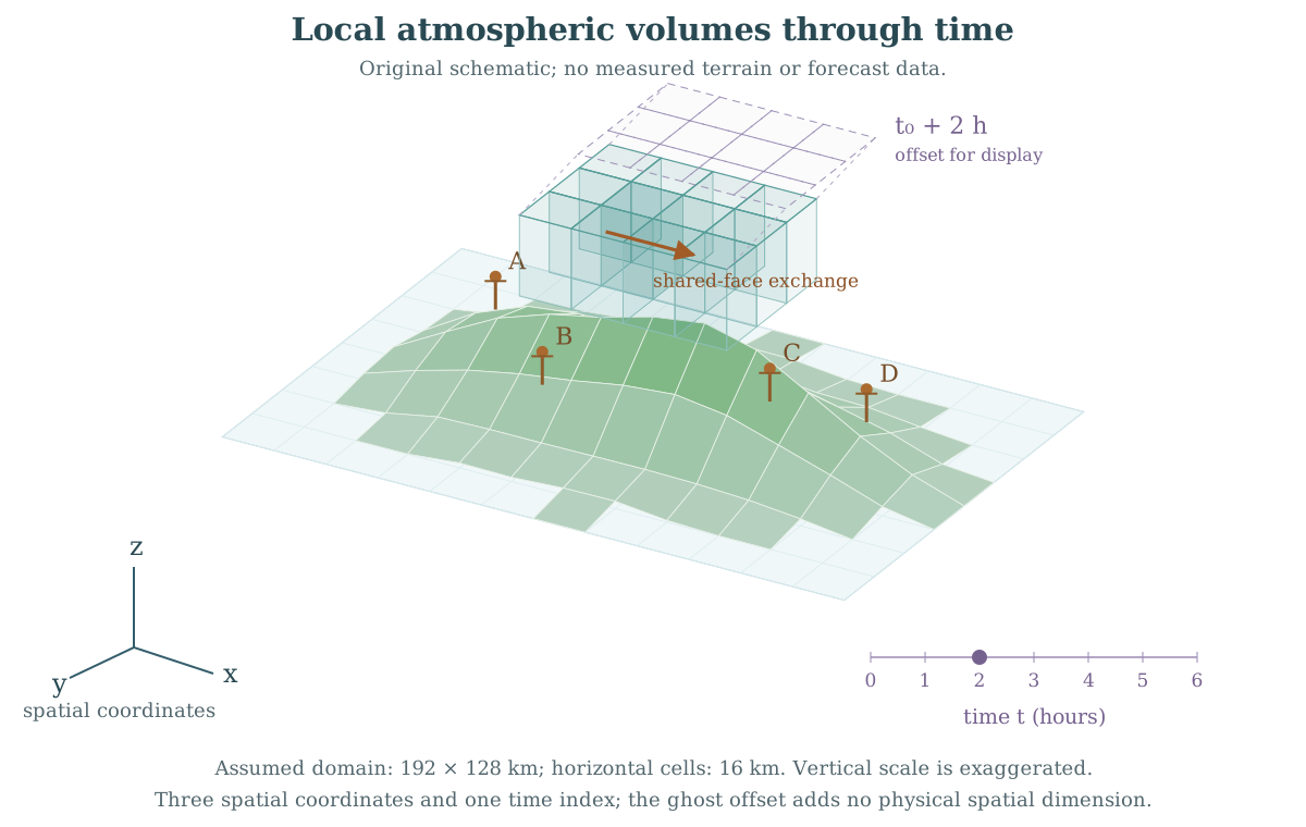
Figure 1. Local atmospheric regions in space and time
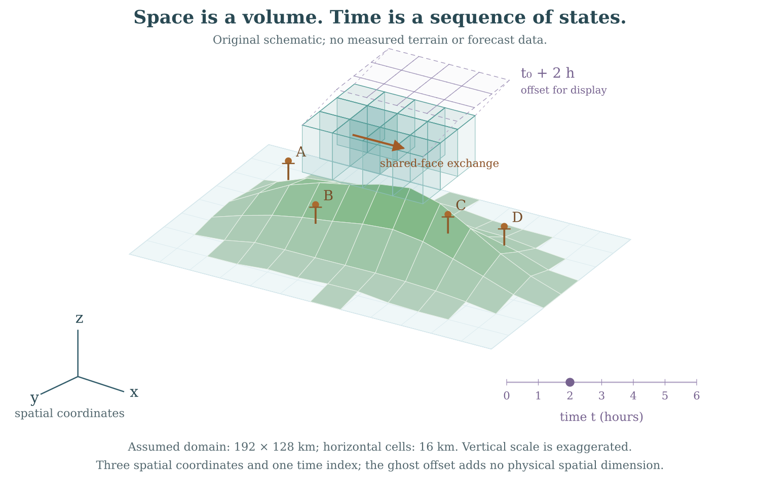
Conceptual geometry for D-LEGOS. Stations, terrain and transport arrows are schematic. A space–time cell is a spatial region crossed with a time interval; it is not a relativistic tesseract or a validated atmospheric simulation.
2.3 Weather events and climate response
Regional hazard studies establish why extremes matter, but they do not collapse weather prediction and climate projection into one task. High-resolution Caribbean cyclone modelling, work on changing shear and sea-surface temperatures, and rapid-intensification analyses address related but different quantities [29; 45; 9]. A model may estimate the intensity of an observed cyclone from imagery, predict its evolution from an initial state, or describe changes in the distribution of cyclone activity under forcing. These are different conditional questions with different validation requirements.
The proposed use of Hurricane Beryl is therefore best framed as a process-oriented event case. It can reveal whether a regional model reproduces circulation, moisture organisation and rainfall under a demanding observed sequence. It cannot by itself establish multi-decadal climate fidelity or future extreme-event return levels. The connection to climate physics can instead concern how transport and stability constrain rainfall across observed regimes. A separate claim about climate-change response would require evaluation of distributions and altered forcing. A visually compelling event reconstruction can motivate the thesis; it cannot stand in for its validation.
Ramseyer and Miller’s Caribbean flash-drought analysis broadens the hazard question beyond heavy rainfall [66]. Their evaporative-demand-based definition identifies rapid drying with subregional structure, rather than one uniform Caribbean event. The physical implication is that rainfall alone cannot characterise every relevant hydroclimatic hazard. Temperature, humidity, radiation and wind can influence atmospheric demand, while the transferability of a drought definition needs its own justification. This supports a multivariable atmospheric state but does not require the initial D-LEGOS experiment to solve both drought and hurricane prediction. A focused benchmark should establish a mechanism before the application portfolio expands.
2.4 What the regional studies establish together
Taylor, Enfield and Chen identify a seasonal change in the ocean regions associated with Caribbean rainfall [76]. Their early-season emphasis on tropical North Atlantic anomalies differs from the stronger late-season role of the equatorial Pacific and Atlantic gradient. This is evidence against fitting a single unconditioned ocean–rainfall relation across the entire rainy season. It is not evidence that sea-surface temperature alone determines convection: the statistical associations need to be interpreted through the circulation and atmospheric state.
Muñoz and colleagues supply part of that physical connection [61]. Their analysis of 1979–2001 reanalyses identifies winter and summer low-level-jet maxima near 925 hPa and connects the midsummer rainfall minimum with enhanced moisture-flux divergence. The diagnosed object is a vertically structured circulation, not simply an island-wide wind-speed index. Read with Taylor and colleagues, this suggests that seasonal ocean associations may act through changes in the transport and stability environment. Their different methods matter: a reanalysis budget diagnosis contains dynamical structure but inherits the reanalysis system, whereas an ocean–rainfall association is more directly a statistical relationship. Neither, alone, establishes a uniquely observed causal chain.
Clarke and colleagues revisit the early-season relationship under a changing atmospheric background [22]. Their comparison over 1979–2024 associates diminished usefulness of absolute sea-surface temperature with changes in stability and circulation. The apparent disagreement with earlier SST-based predictability is therefore not simply that one study is right and the other wrong. The periods, atmospheric background and predictor definitions differ. A relationship useful within a historical regime can weaken when the convective environment changes. This motivates reconstruction and evaluation conditioned on circulation and stability, rather than interpreting a historically important predictor as an invariant control.
Island-scale evidence adds a separate qualification. Sobel and colleagues compare rainfall over tropical islands with the surrounding ocean, separating frequency, intensity and topographic relief [70]. Their subsequent correction changes statistics after removing invalid negative retrieval values [71]. The corrected evidence supports testing island–ocean and terrain contrasts; it does not justify a simple universal island-size threshold for rainfall influence. Together, these studies make observational processing and the physical definition of a regional contrast inseparable.
Table 1 Regional evidence and its limits for atmospheric reconstruction
| Study | Evidence and setting | Established finding | Limit for this thesis |
|---|---|---|---|
| Taylor et al. [76] | Seasonally separated Caribbean rainfall and tropical ocean variability. | Atlantic and Pacific associations differ between the early and late rainfall seasons. | Associations require a circulation pathway; they do not uniquely identify moisture transport. |
| Muñoz et al. [61] | Reanalysis diagnosis of the Caribbean low-level jet and moisture transport. | Seasonal jet structure and moisture-flux divergence connect circulation to rainfall seasonality. | A dynamically coherent reanalysis diagnosis retains reference-system uncertainty. |
| Clarke et al. [22] | Historical early-season rainfall relationships under a changing thermal and circulation background. | Absolute tropical Atlantic temperature loses predictive usefulness as the background changes. | Changed predictor relationships do not alone determine which reconstructed state is correct. |
| Sobel et al. [70; 71] | Satellite island–ocean rainfall contrasts, interpreted with the published correction. | Island relief and rainfall frequency and intensity require separate comparisons. | Retrieval cleaning alters statistics; a universal island-size threshold is unjustified. |
| Campbell et al. [17] | Caribbean regional projections conditioned on global warming levels. | Subregions require separate interpretation of rainfall and temperature changes. | Scenario results are conditional simulations, rather than independent historical state observations. |
| Ramseyer and Miller [66] | Evaporative-demand flash-drought classification across the pan-Caribbean. | Rapid drying has recurring subregional structures; rainfall alone is incomplete. | A drought definition and its support cannot be transferred unchanged to heavy-rainfall reconstruction. |
These findings converge on a specific reconstruction target. A meaningful regional state should preserve the relationship between humidity, circulation and their spatial derivatives across land–sea and terrain boundaries. They do not establish that every component of that state is independently identifiable. The literature thus motivates both a coupled atmospheric representation and an explicit account of the information supplied by observations, background dynamics and assumed source terms.
3 Observations reference products and uncertainty
3.1 Rainfall products represent different information
The CHIRPS data paper describes a precipitation record constructed from infrared information, climatology and station data [33]. This combination is valuable for long regional analyses, including work on persistence and trends in Jamaica [8]. It also means that CHIRPS is an estimated, blended product rather than an independent measurement at every grid point. If the model is trained on CHIRPS and evaluated against stations contributing to that product, the dependence must be recognised. The same station cannot silently serve as both part of the target-construction process and fully independent verification.
The choice of accumulation interval changes the question. Monthly rainfall downscaling can investigate spatial allocation, seasonal structure and consistency with coarse totals. It cannot establish subhourly convective initiation or short-lived rainfall extremes. Conversely, a nowcasting experiment may evaluate event displacement and heavy-rainfall detection without providing the long record required for a climate-trend assessment. The data design should follow the intended claim. Retrieval, temporal forecasting, spatial refinement and climate emulation therefore address distinct evidential questions even when they use the same rainfall archive.
Caribbean evaluations of gridded precipitation products are important because a globally developed product can perform differently across local regimes [20]. Agreement with one reference field can reward the reproduction of that product's errors. A stronger evaluation compares several products, investigates discrepancies by season and terrain, and uses withheld station observations where feasible. Disagreement should be analysed, not averaged away. Where independent observations are absent, the result should be described as reference-product fidelity with a clearly stated observational uncertainty.
3.2 Satellite retrieval and observational operators
Satellite instruments do not directly observe every prognostic variable that an atmospheric model evolves. Infrared cloud information, microwave radiances, optical land-surface reflectance and thermal emission have different relationships to rainfall, humidity and temperature. The precipitation-retrieval literature, including neural bias correction, microwave retrievals and GOES-based conditional models, shows that the observation-to-variable transformation is itself a modelling problem [63; 42; 74]. Its uncertainty should not disappear when the retrieved product becomes an input to another model.
This matters especially when satellite representations are added to D-LEGOS. AlphaEarth and related Earth-observation representations offer reusable information about surface conditions [15; 64; 73]. Yet a model can appear to predict temperature from embeddings partly because temperature-related products entered pretraining. The pretraining inputs and dates therefore belong in the information-set audit [15]. The relevant ablation is not simply with and without embeddings. It is whether the representation adds information beyond the climate variables, dates and geographical signals already available to the baseline, without carrying the evaluation target through an earlier training stage.
Surface skin temperature, near-surface air temperature, sea-surface temperature and sea-level height must remain separate quantities. The literature on satellite temperature downscaling and coastal retrieval makes those distinctions operational [86; 2; 87]. The temperature quantities may share kelvin units while describing different measurands; sea-level height has a length dimension. Their physical definitions and observation operators differ. Sea-level height can reflect mass and steric effects; sea-surface temperature affects surface heat exchange and atmospheric stability through another pathway [58]. A coupling scheme that labels both as a generic ocean feature loses the physical interpretation needed to test its contribution.
3.3 Reanalysis and the meaning of a reference state
ERA5 combines a forecast model with data assimilation to estimate an evolving atmospheric state [44]. It is valuable for constructing multivariable three-dimensional training and evaluation fields. It is not a complete set of independent observations. A learner trained on ERA5 may reproduce its balanced structures and its errors. Comparing that learner with another ERA5-derived field therefore measures a form of model agreement, not an independent test of atmospheric truth.
Temporal information is equally important. A retrospective reanalysis can use information that was unavailable at the issue time of an operational forecast. A smoothing method may legitimately use observations later than the reconstructed state. A prospective forecast may not. This distinction concerns the information available to the inference, not merely the direction of the time index. The same atmospheric sequence can support a sound reconstruction experiment and an invalid forecasting experiment if the information set is not controlled.
Product version, latency, spatial support, accumulation interval and missing-data treatment define the information available to the inference. Filling a missing satellite value with a later observation can be appropriate for retrospective gap filling while introducing leakage in forecasting. Regridding can also change conservation properties. These choices belong in the scientific record because they determine what the model could have known and what its scores actually mean.
3.4 Agreement between products and independent evidence
The observation problem is not solved by selecting the product with the longest archive or finest nominal spacing. Funk and colleagues construct CHIRPS by blending information sources to improve precipitation estimation [33]. That construction supports long regional analyses, but it means that validation against contributing gauges can share information with the target. Avalon Cullen and Al Suhili examine rainfall variability using that product in Jamaica [8]; the resulting trend or persistence analysis is consequently evidence about a particular reconstructed precipitation record, with its processing and observational support.
Centella-Artola and colleagues compare gridded precipitation products against Caribbean gauge observations [20]. Such a comparison addresses a question that a single-product experiment cannot: whether apparent regional features depend on the estimation system. It still requires attention to gauge quality, coverage and overlap. The distinction between a product's agreement with available stations and its accuracy at unobserved sites is especially important where terrain and coastlines are poorly sampled. A product ranking is conditional on the reference network, temporal aggregation and spatial support, rather than a universal ordering of truth.
ERA5 provides another kind of information: a model–observation synthesis with multivariable dynamical structure [44]. It is useful for relating humidity, winds, pressure and temperature consistently, but its internal consistency does not make its fine-scale structures independent measurements. In a reconstruction experiment, ERA5 can serve as a background, a simulation-based truth for controlled tests, or a reference product for comparison. Those roles lead to different claims and cannot be combined without distinguishing them.
The retrieval studies show a related dependency from the observational side. Passive microwave retrieval, infrared estimation and learned bias correction each introduce a relationship between the instrument signal and the target quantity [63; 42; 74]. The resulting product is already an inference. Treating it as an exact observation can transfer retrieval error into a second model while understating uncertainty. The observation operator therefore needs to express the quantity and its support, not merely map one array to another.
Table 2 Observation support and inferential dependence
| Evidence | Measured or estimated quantity | Principal dependence | Defensible use |
|---|---|---|---|
| CHIRPS [33] | Estimated precipitation over a grid cell and accumulation interval. | Blends station and remotely sensed information; contributing gauges may overlap validation. | Precipitation reference with explicit version, support and gauge-overlap audit. |
| Caribbean product evaluation [20] | Gridded rainfall agreement with available gauge observations. | Conclusions depend on gauge coverage and the comparison support. | Regional product sensitivity, rather than a universal product ranking. |
| ERA5 [44] | Assimilated multivariable atmospheric state. | Forecast model, assimilated observations and parameterised processes. | Background or controlled reference-system truth; independent validity needs external evidence. |
| Satellite rainfall retrievals [63; 42; 74] | Rainfall inferred from radiances or imagery. | Retrieval assumptions and common instrument inputs can correlate errors. | An observation operator with footprint, interval and error model. |
| Temperature mappings [86; 2] | Ocean temperature, skin temperature or near-surface air temperature. | Shared units do not make the physical quantities interchangeable. | Variable-specific mapping with exposure, height and surface conditions stated. |
| Sea-level estimate [58] | Height changes influenced by mass and steric contributions. | Length is dimensionally distinct from temperature; mechanisms differ. | A separately justified ocean covariate, rather than a substitute for sea-surface temperature. |
A useful synthesis follows. The availability of several products permits sensitivity analysis, but agreement among them is not automatically independence when they share observations or algorithms. Their disagreement can expose uncertainty; their agreement may partly reflect common inputs. For the present research question, the strongest evaluation separates reference-product fidelity from skill against genuinely withheld evidence and reports where independent validation remains unavailable. This is a limit on what can be inferred, not a reason to dispense with reanalysis or satellite estimates.
Explainer · The thermometer and the photograph
Suppose you want to know the temperature of the air beside a road. A thermal image of the road measures something different: the radiating surface. Both may be reported in kelvin, but shared units do not make them the same measurement. An observation operator is the explicit bridge from the atmospheric quantity being reconstructed to the quantity the instrument reports. The same reasoning applies when a rainfall retrieval, station measurement and reanalysis value disagree. Agreement must be assessed at comparable spatial support, height and time. [44]
The observation review requires explicit product versions. CHIRPS3 updates the climatology, station information and treatment of precipitation variability relative to CHIRPS2, while retaining a 0.05-degree land grid and extending the geographic domain. The 2015 methods reference remains appropriate for CHIRPS2; it cannot alone document a CHIRPS3 analysis. IMERG likewise requires its version and run designation because Early, Late and Final products differ in available information and latency. Retrospective training against a delayed Final product can answer a useful reconstruction question, but treating that product as available at forecast issuance would overstate operational feasibility. These changes also complicate apparent model progress: a result can improve because the reference product changed. A reproducible Caribbean evaluation should freeze dataset identifiers, acquisition dates, accumulation intervals and processing, then test whether the scientific conclusion survives reasonable reference-product choices. [33; 106; 107]
4 Regional modelling and learned downscaling
4.1 Emulation is a conditional claim
An emulator approximates the behaviour of a specified parent model under a specified set of inputs. It does not automatically improve that model's agreement with observations. Doury and colleagues establish a regional-emulation approach in which a neural network learns aspects of the downscaling relationship represented by a regional climate model [27]. Work comparing training frameworks and examining transferability shows why the predictor source matters [79; 11; 43]. An emulator trained with upscaled regional-model fields may face an easier problem than one driven by a distinct global model carrying structural biases.
This distinction affects the interpretation of a successful super-resolution experiment. If a fine field is averaged and the average is supplied as input, the coarse target is exactly consistent with the desired fine output. Real global-model inputs need not have that property. They may place a storm incorrectly, distribute moisture differently or produce a biased regional total. The test therefore needs to distinguish a perfect-prognosis experiment from an imperfect-driver experiment. Both are useful, but they answer different questions.
Classical climate emulation also deserves attention. Statistical emulators and reduced-dimensional representations map forcing or model parameters to climate responses without claiming to resolve atmospheric evolution at every grid point [77; 46; 56]. Such methods are relevant baselines for regional mean responses and uncertainty exploration. They are less suitable for detailed event trajectories, but their simplicity can be an advantage when the target is an aggregate climate statistic. The choice between a statistical emulator and a learned dynamical model should follow the target, not a presumption that the more elaborate architecture is scientifically superior.
4.2 Deterministic refinement and strong simple alternatives
DeepSD established an early super-resolution approach to climate downscaling [80]. Later comparisons of neural configurations with traditional downscaling methods provide a more informative basis for model selection than isolated demonstrations [10]. Their shared lesson for D-LEGOS is methodological: model complexity should be judged against statistical alternatives using the same information, splits and target variables. A neural model that outperforms a weak interpolator has not necessarily improved on a well-designed seasonal or topographic regression.
Deterministic mean-squared-error training favours the conditional mean. When several fine-scale rainfall configurations are compatible with the coarse input, averaging them can produce a smooth field. That smoothness is not merely an aesthetic failure. It can suppress local intensities and alter the spatial structure relevant to flooding. However, sharpness should not be treated as a corrective metric in isolation. A sharp rainfall cell in the wrong location can be less useful than a calibrated probability of heavy rain over the relevant catchment.
Geostatistical and area-to-point methods provide another useful comparison [87]. They make spatial support and aggregation explicit. For the doctoral programme, these methods are valuable because they help separate a genuine advantage of learned features from an advantage obtained through a different treatment of grid-box averages. The baseline set should include methods that use terrain and seasonality well, rather than only methods chosen because they are easy to outperform.
4.3 Generative downscaling and distributional credibility
Generative methods model several plausible fine-scale outcomes conditional on coarse information. Adversarial precipitation downscaling and stochastic super-resolution demonstrate why coherent spatial samples can be useful [41; 53]. Diffusion methods extend this line through iterative conditional generation and residual refinement [4; 55; 1]. Their outputs should be evaluated as samples from a conditional distribution. Scoring a single attractive sample, or comparing an ensemble mean with an individual deterministic field, can obscure what the method is designed to represent.
Lopez-Gomez and colleagues combine dynamical downscaling to an intermediate resolution with generative refinement [55]. This is a close conceptual ancestor of a hybrid regional framework. It establishes that combining a numerical model and a generative model is already a developed research direction. The D-LEGOS contribution must therefore be more specific: for example, whether explicit local coupling and uncertainty-aware constraints improve reconstruction and generalisation in island environments under controlled comparisons. Application to Jamaica can make the scientific test important, but the geographical change alone is insufficient evidence of a new method.
Aich and colleagues combine downscaling with bias correction [4], while transferability studies examine the difficulty of applying learned relationships under changed conditions [11; 43]. These studies place a requirement on any climate application: improved historical spatial statistics must not erase or distort the parent model's climate-change response without an explicit reason. Conversely, exact reproduction of a parent-model change is not necessarily the goal if the parent is known to be biased. The thesis must state whether it seeks faithful emulation, observational adjustment or a new physical prediction. Those objectives cannot be evaluated with one undifferentiated score.
4.4 Driver error changes the meaning of successful downscaling
The studies of Doury and van der Meer illustrate why the definition of an emulator matters. Doury and colleagues learn daily near-surface temperature fields associated with a specified regional model, using a European configuration at approximately 12 km [27]. The target is a particular downscaling relation, not a complete replacement atmosphere. The paper's discussion of temperature extremes, climate-change intensity and transfer to different models limits how a successful emulation should be generalised. A low error for one surface variable does not establish a correct moisture budget or performance over Caribbean terrain.
Van der Meer and colleagues use Antarctic Peninsula surface mass balance to compare perfect and imperfect training frameworks [79]. When the coarse input is obtained from the same regional simulation as the fine target, the learner primarily faces a resolution-recovery problem. Replacing that input with a distinct global model changes the distribution and exposes model inconsistencies. The reported underestimation under that transfer, and the improvement from training with imperfect-model inputs, provide direct evidence that driver provenance changes the task. The lesson is methodological rather than geographic: it does not transfer Antarctic surface-mass-balance performance to Caribbean rainfall.
Harris and colleagues make a related distinction in stochastic precipitation downscaling [41]. Their framework addresses forecast error as well as spatial refinement, using independent forecast inputs and a precipitation reference. Distributional verification, including calibration and spatial structure, is therefore more appropriate than judging one visually sharp output. A conditional mean and an ensemble of possible fields answer different statistical questions. The comparison with coarsen-and-recover designs explains why an apparently excellent super-resolution score can be insufficient for a practical atmospheric inference task.
Harder and colleagues address consistency at the output of a downscaler [40]. Their constraint layers include additive, multiplicative and other normalising constructions. These make designated relationships exact, a property that differs from a penalty that is merely encouraged during optimisation. Their experiments demonstrate useful performance in the evaluated settings, but an algebraic constraint cannot determine whether the imposed coarse total is observationally correct. The uncertainty of the driver remains a scientific question after the numerical constraint has been satisfied. Their multiplicative construction also exposes a practical distinction between different hard constraints: division by a small predicted average can be unstable, and positivity requires appropriate restrictions. The softmax construction enforces non-negativity as well as the selected average when its coarse input is admissible. These choices change the feasible output and numerical behaviour; they are not interchangeable ways of adding a generic conservation label [40].
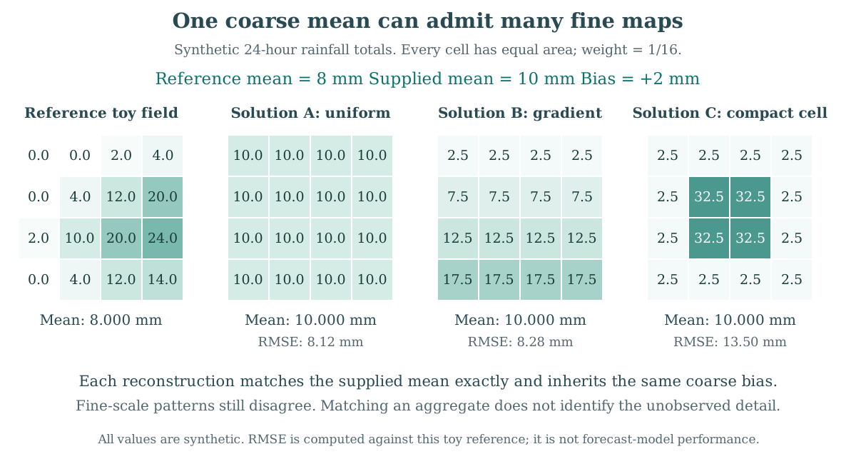
Figure 2. Many fine fields can share one coarse average
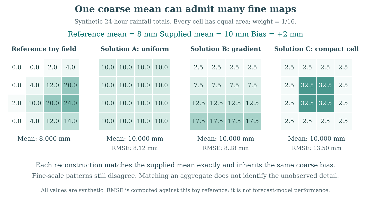
An equal-area synthetic example. The fine fields satisfy the supplied coarse mean by construction. Changing the coarse bias demonstrates that exact aggregation can preserve an incorrect total. This is an explanatory calculation, not a reproduction of Harder et al. [40].
Explainer · A holodeck can look convincing
A fictional holodeck could generate several convincing storms from the same coarse weather description. A generative model also supplies possible fine-scale states conditional on its information. Looking realistic is useful evidence about appearance, but it does not tell us whether the generated storm occurred. The scientific checks concern probabilities, extremes, location, dependence and physical budgets. A family of plausible outcomes should remain a family until observations discriminate among them.
Table 3 Close downscaling precedents answer different questions
| Study and task | Data and physical treatment | Comparison and finding | Bounded implication |
|---|---|---|---|
| Doury et al. [27] Regional emulation | Daily near-surface temperature from a specified European regional model; learned refinement. | Learns its regional-model relationship; extremes and transfer delimit generalisation. | Surface-variable fidelity does not establish multivariable atmospheric recovery. |
| van der Meer et al. [79] Driver dependence | Antarctic surface mass balance; perfect and imperfect model training frameworks. | Changing to independent coarse inputs exposes bias; imperfect-framework training changes performance. | Driver provenance must be controlled before attributing gains to constraints. |
| Harris et al. [41] Stochastic precipitation | Forecast inputs and precipitation reference; conditional generative refinement. | Contrasts practical forecast downscaling with coarsen-and-recover designs; evaluates distributional behaviour. | Forecast error and unresolved fine-scale variation are distinct uncertainties. |
| Harder et al. [40] Exact constraints | Coarse and fine fields with algebraic constraint layers, including additive and multiplicative forms. | Designated aggregation relationships hold exactly; predictive performance is evaluated separately. | A correct constraint can transmit an incorrect coarse total. |
| Lopez-Gomez et al. [55] Dynamical and generative refinement | Intermediate dynamical downscaling followed by generative refinement of climate ensembles. | Compares distributional and multivariate structure with statistical alternatives. | Hybrid downscaling is an established lineage; its evidence does not establish D-LEGOS novelty. |
| Das et al. [23] Extreme nowcasting | Tennessee Valley radar-based NowcastNet; physics-conditioned generation. | Heavy-rainfall detection improves against HRRR, advection and persistence; aggregate bias persists. | Detection skill and water-volume error can disagree; regional transfer remains untested here. |
These papers resolve different parts of the same difficulty. Doury establishes a learned regional-model relationship; van der Meer exposes the effect of imperfect coarse inputs; Harris treats conditional variability and forecast error; Harder controls selected consistency properties. They do not establish one universally preferable architecture. Their joint implication is that the contribution of a physical constraint must be separated from the advantage of a cleaner driver, a different target or a different information set. That comparison is directly relevant to D-LEGOS, whose proposed coupling will otherwise be difficult to interpret independently of its inputs and loss design.
CorrDiff's conditional-mean and stochastic-residual decomposition demonstrates how downscaling can recover variability suppressed by deterministic regression, while its reported calibration limitations show why visual realism is insufficient. A related problem is whether a sequence of individually plausible fields preserves temporal dependence. EnScale-t addresses that problem by conditioning daily downscaled fields on the previous day and evaluating temporal structure alongside multivariate dependence and calibration. Its Central European climate-model setting differs from CorrDiff's Taiwan analysis targets, so it supplies methodological evidence rather than a direct performance ranking. The published EnScale study also limits the interpretation of its extrapolation test: training extends to 2089 and testing on 2090–2099 represents only a modest departure. For D-LEGOS, temporal consistency should be measured rather than inferred from an animation, and successful statistical dependence should remain distinct from demonstrated conservation across physical interfaces. [102; 112]
5 Learned atmospheric evolution and climate emulation
5.1 Global forecast skill and regional relevance
GraphCast, Pangu-Weather, FourCastNet, FuXi and AIFS demonstrate distinct learned representations of atmospheric evolution [51; 12; 62; 21; 52]. Graph-based, spectral and transformer methods should not be treated as interchangeable implementations. They encode spatial interaction differently and can respond differently to geometry, variable scaling and autoregressive error. Nevertheless, their common relevance is that the mapping between analysed atmospheric states can be learned well enough to provide serious weather-prediction comparators.
For a Caribbean PhD, the central question is what those comparisons leave unresolved. Global aggregate performance can conceal errors near small islands, in heavy precipitation or within poorly observed boundary layers. A model trained on reanalysis may provide an excellent large-scale driver while still requiring a local observation model and regional evaluation. Comparing D-LEGOS with these systems is useful only when the target, initial state, horizon and verification source are aligned. A regional model should not be rewarded for seeing later observations or finer targets unavailable to the global comparator.
Bonavita’s examination of early machine-learning forecast systems identifies limitations in fine-scale variability and physical consistency in the evaluated model versions. It supplies a reason to diagnose physical structure alongside aggregate skill, not a universal verdict on later learned forecasting systems. [105]
Aurora broadens the discussion from one fixed forecast task to transferable Earth-system representations [14]. AlphaEarth addresses a different representational problem, primarily associated with Earth-observation information [15]. Conflating them would obscure the difference between a learned representation of surface properties and a prognostic atmospheric model. Both may supply useful components, but each component requires a specific hypothesis about the information it adds and the physical quantity it helps estimate.
GenCast strengthens the case for treating atmospheric prediction as a conditional distribution. Its published evaluation uses global ensembles at 0.25-degree resolution, twelve-hour steps and a fifteen-day horizon. However, the reported advantage across 1,320 verification targets concerns combinations of variables, lead times and vertical levels; those targets are dependent and do not represent 1,320 independent forecasting problems. More directly relevant to this review, the authors exclude precipitation from their main scorecard because of concerns about ERA5 precipitation quality. The result therefore cannot support a claim that GenCast has already solved Caribbean rainfall prediction. Its contribution is an ensemble methodology and a documented verification design that can inform a regional experiment. Such an experiment still needs rainfall observations, local thresholds and an evaluation of whether predictive probabilities remain calibrated over the target domain. [99]
5.2 Observation-driven models and input availability
Direct observation-to-forecast systems address a limitation of analysis-initialised learners: dependence on the analysed state and its latency [72; 7; 6]. WeatherNext 3 is a recent source in the collection that explicitly addresses observational input and resolution [68]. Its title and preprint status should not be used to infer that weights, archives, operational access or Caribbean coverage are automatically available. Those are separate implementation questions. The literature supports a comparator design; actual access must be verified at the time of experimentation.
The satellite nowcasting literature makes latency especially concrete [3]. A high-resolution product arriving after a forecast issue time is unavailable as an operational predictor for that issue. Likewise, a retrospective archive of fixed-lead forecasts is not necessarily a single uninterrupted trajectory from one initialisation. The experiment must retain forecast reference time and valid time, not just a date and a lead label. These details determine whether the model is learning a forecast relationship or benefitting from retrospective data assembly.
DGMR and NowcastNet address related prediction difficulties through distinct modelling choices. DGMR produces probabilistic radar sequences, with evaluation that combines statistical performance, economic measures and meteorologist assessment. NowcastNet conditions generative predictions on physical evolution of the precipitation field. The reported studies establish these approaches in radar-rich settings, with different forecast horizons and evaluation protocols. They do not justify ranking the architectures from a single number collected across separate papers. Nor does evolution of a radar-derived rain field amount to solving the complete moist atmospheric system. Transfer to Jamaica would change the evidence base if satellite retrievals or sparse stations replace dense radar sequences. Observation resolution, latency and retrieval uncertainty must then be treated as part of the task definition. The appropriate extension is a matched regional comparison that isolates architecture from differences in available information. [100; 101]
Das and colleagues provide a particularly instructive hybrid physics–AI nowcasting comparison [23]. Their evaluation of NowcastNet against HRRR, advection and persistence finds improvements for heavy precipitation in the studied Tennessee Valley setting, while identifying overestimation of spatially aggregated rainfall at longer leads. The strength of this result lies in the defined event and comparator evaluation, not in a general claim that AI has superseded numerical prediction. Its limitation is equally relevant to D-LEGOS: improved grid-cell detection can coexist with an undesirable aggregate bias. Local scores, area-integrated quantities and lead-time behaviour therefore need joint interpretation.
5.3 A close reading of the supplied NowcastNet comparison
Das et al. evaluate NowcastNet against HRRR, persistence and advection in a retrospective Tennessee Valley study involving 30 selected heavy-precipitation events. Forecasts and MRMS quantitative precipitation estimates are compared at common spatial and temporal supports. The study is particularly useful because it reports several verification families rather than one pooled accuracy score. Its event selection, regional radar information and short forecast horizon define the population to which the reported comparisons apply. They do not establish Caribbean transfer, all-weather performance or forced climate response. [23]
The results support a metric-dependent interpretation. Categorical and neighbourhood scores reward the detection and placement of rainfall above a chosen threshold. Continuous-error and aggregate diagnostics expose a different weakness: the paper reports overprediction of rainfall as the horizon increases, with HRRR performing better at two to three hours on the reported RMSE, inverse-NMSE and normalised-error comparisons. A model can therefore produce more useful evidence that heavy rain will occur while estimating its amount less accurately. For regional moisture reconstruction, this is a reason to evaluate event detection and area-integrated budgets together. [23]
The supplied article also requires care when numerical findings are illustrated. Its abstract reports a median CSI pair for a heavy-rain threshold without specifying a lead time, and that attribution does not readily reconcile with the corresponding boxes in Figure 4 on visual inspection. The review does not reconstruct exact numbers from the plotted boxes or use the abstract pair as a headline performance chart. The discrepancy remains an author-clarification or raw-score check. The qualitative lead-time and metric trade-off is supported separately by the main text and figures. The supplement was not retrieved in this update. [23]
NowcastNet’s transport-and-growth formulation is scientifically instructive, but the transported precipitation proxy is not the full atmospheric water inventory. A complete three-dimensional water budget also involves density, water vapour, condensate, boundary transport, evaporation, precipitation and unresolved processes. The schematic advection equation used in the animation below is written explicitly as ∂R/∂t + v·∇R = S^R; it is the review’s explanatory notation. It does not certify conservation of atmospheric water, momentum or energy. [23; 101]
Figure 3. Transport and growth are different parts of a rainfield
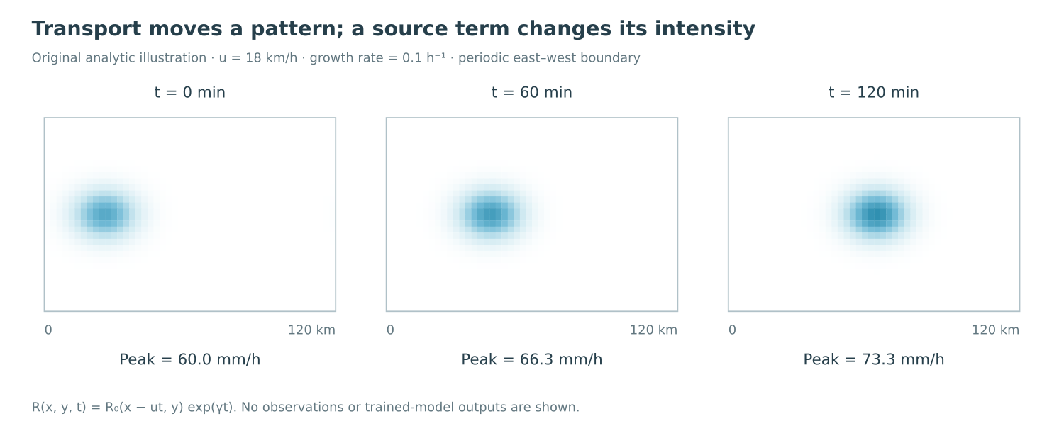
Analytically prescribed synthetic rainfall, inspired by the transport–evolution distinction in NowcastNet. The animation is not a trained forecast or a reproduced event from Das et al. [23].
5.4 Climate stability requires a different test
Weather skill does not establish climate fidelity. ACE and ACE2 address long integrations, boundary conditions and forced responses more directly than short-range forecast benchmarks [84; 85]. The E3SMv2 emulator assessment focuses attention on precipitation behaviour during extended simulation [30]. LUCIE addresses computationally manageable ensemble emulation [38]. Together these studies make long-run distributions, variability and physical drift part of the validation target rather than optional extensions to a forecast score.
NeuralGCM provides a different hybrid design by combining a differentiable dynamical core with learned parameterisations [49]. It offers a close precedent for preserving resolved dynamics while learning unresolved tendencies. Its relevance to D-LEGOS is therefore both constructive and limiting. It supports the value of combining physical evolution and learning, but it prevents the generic phrase physics-informed climate model from serving as a novelty claim. The thesis needs to identify which physical process, interface formulation or inference problem is improved, under which observations and approximations. The accessible NeuralGCM study supplies a useful internal comparison: its large-scale hydrostatic solver is coupled to learned column tendencies, rather than replaced by a residual-trained regional neural field. Its historical sea-surface-temperature-forced integrations and its warmer-SST experiments answer different questions. In the examined perturbations, response under modest warming is more credible than under the larger warming perturbation, where the response diverges from expectations. The existence of a dynamical core thus strengthens physical structure without establishing arbitrary extrapolation. This is a more specific reason to separate historical reconstruction from climate-response claims [49].
Ocean emulators and coupled hybrid ocean frameworks further show that an apparently successful component may behave differently when coupled [31; 24; 88]. A local atmospheric network that reproduces an offline tendency can destabilise a coupled rollout if its errors feed back into humidity, surface exchange or neighbouring blocks. Long-run stability is thus a property of the interacting system. It cannot be certified by validating each module separately.
The precipitation-focused NeuralGCM study published in 2026 provides a more direct precedent for learning from observations while retaining physical accounting. Yuval and colleagues train the differentiable hybrid model against IMERG precipitation at 2.8-degree resolution. The inspected preprint describes a learned precipitation module with evaporation diagnosed through the column-water budget, and it explains that ERA5 moisture variables and IMERG rainfall can impose conflicting training targets. This is a consequential limitation: enforcing a budget does not establish which observational estimate is correct, and model optimization must accommodate disagreement between products. The paper also distinguishes formulations that conserve column water from formulations that ensure non-negative precipitation. For D-LEGOS, observational supervision, conservation and admissible state bounds should therefore be evaluated as separate properties. Their combination is established prior art; a doctoral contribution would need a more specific advance in regional coupling, numerical behaviour or verified predictive performance. [103]
Independent hierarchical assessment provides a useful complement to forecast benchmarks. Chen and colleagues examine NeuralGCM through synoptic tests, ENSO-related interannual responses and idealized uniform-warming experiments. The retrieved publication abstract reports both plausible behaviour and deficiencies, including nonlinear teleconnection responses and differences in upper-atmospheric warming and circulation. These findings support a graded interpretation of model credibility. A model can reproduce one class of atmospheric behaviour without establishing competence across all forcing regimes. For the proposed Caribbean system, this motivates separate tests of local conservation, complete storm sequences, seasonal rainfall distributions and controlled changes in boundary conditions. Uniform warming is a diagnostic perturbation rather than a verified future scenario. Because only the abstract and indexed conclusion were inspected for this recent study, its detailed numerical results should remain outside the present synthesis until the full methods and supporting analyses have been examined. [104]
6 Physics informed learning and the meaning of a constraint
6.1 Governing residuals and unresolved processes
The PINN formulation associates a learned field with residuals of a differential equation and its initial or boundary conditions [89]. Physics-informed neural operators extend the idea towards learning families of solution maps, sometimes applying physical residuals at a resolution different from the training data [54]. These are useful methodological distinctions. A PINN commonly approximates a field for a specified problem instance; an operator learner aims to generalise across functions or initial conditions. Their computational cost and generalisation tests should reflect those different objectives.
The broader physics-informed learning literature includes equation penalties, architectural constraints, operator regression and hybrid numerical solvers. This taxonomy is useful because the location at which physics enters a model determines which relationship is encouraged or guaranteed and which empirical comparison remains necessary. [90]
An atmospheric residual is meaningful only after the state and approximation are specified. Moist convection, radiation, turbulent transport, surface exchange and phase changes can be unresolved at the chosen grid. Their absence from the resolved equation does not imply their absence from the atmosphere. If a neural field is penalised for violating an incomplete equation, the optimisation can force it towards the wrong solution. Learned closure terms may be necessary, but they must have defined units and physically interpretable roles. A residual made small by a freely adjustable source term does not demonstrate that the relevant physical mechanism has been learned.
The climate-parameterisation literature makes this problem explicit. Studies of gravity-wave fluxes, moist physics, radiation and coupled ocean components address particular closures rather than an unspecified collection of physical laws [39; 83; 88; 67]. The lesson for D-LEGOS is to start with a defensible subset of balances and a clear account of unresolved tendencies. More equations do not automatically imply more physical credibility. Some may be redundant, inconsistent with the coordinate system or invalid at the selected scale.
ClimODE offers a related atmospheric example with a different scientific target. Verma et al. (2024) represent forecast evolution through a neural ordinary differential equation informed by a transport formulation and add a probabilistic emission model with learned bias and variance. The reported evaluation uses WeatherBench ERA5 fields on a 5.625° grid at six-hour intervals, with training in 2006–2015, validation in 2016 and testing in 2017–2018. Its five target fields are two-metre temperature, the two ten-metre wind components, 850-hPa temperature and 500-hPa geopotential. Surface precipitation is not among them. This evidence establishes a precedent for interpretable transport structure in learned weather evolution at the evaluated support. It does not establish island-scale rainfall reconstruction or a closed moist-atmospheric budget. A continuous transport equation also leaves the conservation properties of the implemented numerical evolution to be demonstrated. ClimODE is consequently useful for comparing what the learned dynamics represent, with its reported forecasting task kept distinct from retrospective inference. [97]
6.2 Hard and soft constraints
Soft constraints enter an objective as weighted penalties. Hard constraints restrict the admissible output, for example by construction or projection. Hard-constrained downscaling supplies a direct precedent for enforcing aggregation consistency between coarse and fine fields [40]. This makes the designated coarse-scale relationship exact within the implemented arithmetic. Positivity is a separate condition and depends on the chosen layer. It does not guarantee that the imposed coarse total is correct, or that the fine-scale allocation is realistic.
Atmospheric parameterisation provides a useful distinction between learning a balance and restricting the admissible output. Beucler et al. (2021) compare penalties on analytic constraints with neural constructions that satisfy selected linear relationships. Their results show why predictive error and conservation require separate diagnostics: imposing a balance does not ensure improvement in every predicted quantity or establish transfer to a warmer climate. For a regional reconstruction, an analogous distinction concerns the water ledger. A penalty on neighbouring outward fluxes leaves a residual determined by training, whereas one shared integrated face transfer cancels from the sum of the two discrete budgets by construction. That cancellation establishes an accounting property. Its physical usefulness still depends on the accuracy of the transfer, the source terms and the external boundaries. Non-negativity, numerical stability and reliable rainfall allocation require their own conditions and tests. The experiment should consequently report both the enforced relationship and independent errors in the reconstructed state. [96; 92]
This distinction is particularly important when coarse fields are biased. An exact constraint can transmit a coarse error to every fine-scale realisation. A soft constraint can permit correction but introduces dependence on weights and optimisation. Neither choice is universally preferable. The scientific comparison should vary coarse-driver bias and observational error, then measure the trade-off between constraint satisfaction and independently verified prediction. The D-LEGOS conservation component is useful insofar as it isolates that trade-off; it cannot establish that the entire atmospheric framework is valid.
The word conservation also requires care. Non-negative rainfall is an admissibility condition. Exact preservation of a coarse monthly rainfall total is an aggregation constraint. A closed water budget relates storage, transport, evaporation, precipitation and other relevant terms over a defined volume and interval. These are not equivalent achievements. The thesis should name precisely which condition is enforced and report it in its physical units. A small normalised loss is not a substitute for an interpretable budget diagnostic.
6.3 Optimisation is part of the physical-method comparison
Wang and colleagues identify unbalanced gradients and numerical stiffness in composite PINN objectives [81]. Krishnapriyan and colleagues show that optimisation can fail even when the network is expressive enough to represent the solution [50]. Causal training methods further emphasise temporal ordering [82]. Together these papers weaken an easy interpretation of a failed physics-informed model: failure does not necessarily show that the physical constraint is unhelpful. It may show that the imposed formulation is difficult to optimise.
Neural tangent kernel analysis further identifies unequal convergence rates among PINN loss components under its stated limiting assumptions. This explains a class of training imbalance; it does not supply a convergence guarantee for finite atmospheric networks. [91]
The converse also matters. A constrained model that receives extensive tuning cannot be compared fairly with an unconstrained model given a default training schedule. Architecture, capacity, data, stopping rules and search budgets should be matched where possible. A useful ablation separates the effect of the equation from the effect of normalisation, curriculum, architecture or longer training. Loss-weight optimisation, including adaptive schemes, should be evaluated against simple schedules before reinforcement learning is introduced. The literature does not make an adaptive controller necessary merely because several losses compete.
Physical interpretability should therefore extend to the training record. The researcher should inspect residual distributions by season, altitude, terrain and event intensity; not only the average loss. A model may fit widespread weak tendencies while neglecting rare but important convective regimes. Similarly, a low total objective can conceal a large error in a physically decisive term if the normalisation or sampling gives that term little influence. These observations support reporting the individual residuals and their scales alongside predictive metrics.
6.4 A physical framework for interpreting the evidence
The atmosphere is a coupled, forced and dissipative system. For regional reconstruction, the choice of governing balances determines which observations can constrain which parts of the state. A useful starting point is a pressure-coordinate representation of horizontal wind u and v, temperature T, specific humidity q and geopotential Φ, together with pressure velocity ω. Geopotential height z is related to Φ by Φ = gz under the usual constant-g approximation; they must not be used interchangeably without their units. Pressure velocity has units of Pa s⁻¹ and is not geometric vertical velocity in m s⁻¹. These apparently modest distinctions are consequential when observations, reanalysis variables and model derivatives are combined.
Under a hydrostatic ideal-gas approximation, using virtual temperature in the density relation, a schematic set of resolved balances is
Equation 1. Resolved hydrostatic atmospheric balances
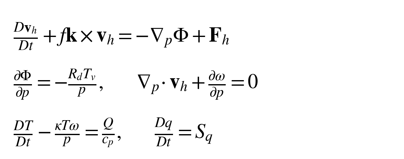
Editable notation: D v_h/Dt + f k×v_h = −∇_pΦ + F_h; ∂Φ/∂p = −R_d T_v/p; ∇_p·v_h + ∂ω/∂p = 0; DT/Dt − κTω/p = Q/c_p; Dq/Dt = S_q.
The balances connect horizontal momentum, hydrostatic pressure support, mass continuity, temperature and humidity. They are schematic resolved equations, with unresolved tendencies explicit. Hydrostatic balance omits vertical acceleration, so a fine output mesh alone cannot justify a convection-permitting claim.
v_h=(u,v) — horizontal velocity; m s⁻¹.
ω — pressure velocity; Pa s⁻¹.
Φ — geopotential; m² s⁻².
T_v — virtual temperature; K.
q — specific humidity; kg kg⁻¹.
Q — diabatic heating per mass; W kg⁻¹.
S_q — net humidity tendency; s⁻¹.
F_h — unresolved momentum tendency; m s⁻².
c_p — specific heat at constant pressure; J kg⁻¹ K⁻¹.
f — Coriolis parameter; s⁻¹.
R_d — dry-air gas constant; J kg⁻¹ K⁻¹.
κ = R_d/c_p — ratio of dry-air gas constant to heat capacity; dimensionless.
T — temperature; K.
p — pressure; Pa.
k — unit vector along the local vertical; dimensionless.
t — time; s.
Here virtual temperature T_v accounts for the density effect of water vapour under the stated approximation; condensate loading requires an additional correction. The horizontal wind is v_h = (u, v), D/Dt = ∂/∂t + v_h·∇_p + ω∂/∂p, f is the Coriolis parameter, Rd is the dry-air gas constant, cp is specific heat at constant pressure and κ = Rd/cp. The horizontal gradient is taken on constant-pressure surfaces. The terms F_h, Q and Sq denote unresolved momentum tendencies, diabatic heating rate per unit mass (J kg⁻¹ s⁻¹) and moisture sources or sinks, respectively. The thermodynamic form displayed treats heat capacities and composition approximately; a moist formulation should state the chosen corrections and condensate treatment. The equations provide an interpretive framework, not a claim that the intended implementation already solves a complete atmospheric model. Their implementation must respect the geometry, boundary conditions and selected approximation regime. The unresolved momentum tendency F_h has units m s⁻² and the specific-humidity tendency S_q has units kg kg⁻¹ s⁻¹. With c_p in J kg⁻¹ K⁻¹, Q/c_p has units K s⁻¹. This simplified pressure-coordinate framework is informed by the governing balances documented in the IFS; that source uses a hybrid vertical coordinate and more detailed moist thermodynamics. [113]
The pressure-coordinate continuity equation links horizontal divergence to vertical mass motion. It does not imply that three independently learned wind components automatically form a mass-consistent flow. Hydrostatic balance constrains the vertical pressure–geopotential relation, but it does not resolve the vertical accelerations of explicit deep convection. At kilometre scales, nonhydrostatic processes can matter. The kilometre-scale Earth-system simulation literature illustrates the physical and computational demands associated with resolving these processes [48]. A hydrostatic reconstruction may still be useful at an explicitly selected scale; it should not borrow the label convection permitting from a different configuration.
Humidity adds another constraint on interpretation. A specific-humidity tendency is not precipitation. The conversion of water vapour to condensate and the conversion of condensate to surface rainfall involve processes and storage not represented by a single advection equation. Likewise, a thermodynamic source term fitted from residual error can absorb several mechanisms with different responses to warming. The learned source may be predictive within a distribution without being physically identifiable. Studies of learned moist physics and radiation provide relevant precedents because they define the processes being emulated and examine coupled stability [83; 67]. They do not remove the need to specify those processes in the proposed regional application.
A column-integrated water balance is especially useful for connecting the physical formulation to the rainfall literature. Neglecting condensate storage and top-of-atmosphere vapour flux, and treating the moving surface-pressure boundary consistently, define precipitable water W and horizontal vapour transport Q_v by pressure integration. The resulting diagnostic balance is
Equation 2. Column water storage and transport
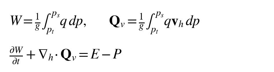
Editable notation: W = (1/g)∫q dp; Q_v = (1/g)∫q v_h dp; ∂W/∂t + ∇_h·Q_v = E − P.
Storage changes when evaporation, precipitation and horizontal transport do not balance. This vapour approximation neglects condensate storage and top vapour flux, and requires consistent treatment of the moving lower pressure boundary. Matching a downscaled rainfall mean does not enforce this atmospheric balance.
W — column water-vapour mass; kg m⁻².
Q_v — vertically integrated vapour transport; kg m⁻¹ s⁻¹.
E,P — evaporation and precipitation mass flux; kg m⁻² s⁻¹.
g — gravitational acceleration; m s⁻².
p — pressure; Pa.
W is measured in kg m⁻² and Q_v in kg m⁻¹ s⁻¹; evaporation E and precipitation P are mass fluxes in kg m⁻² s⁻¹. Dividing the accumulated mass per unit area by liquid-water density converts it to a water-depth accumulation. This accounting makes clear why rainfall aggregation and atmospheric water conservation are different tests. An exact match between a fine-grid monthly rainfall sum and its coarse-grid parent constrains one integrated output. It says nothing by itself about moisture storage or transport, and can hold even if both the coarse and fine estimates are biased.
Regional water-budget closure also involves open boundaries. Integrating over a volume converts the divergence term into a boundary flux. If neighbouring D-LEGOS blocks each estimate their own outward flux at a shared face, their signs and face measures must be reconciled. A conservative exchange should contribute equal and opposite transfers to the adjacent control volumes. A penalty that merely makes humidity values agree on the interface is weaker: flux additionally depends on velocity, density or the selected coordinate measure. Where precipitation or evaporation is prescribed, its uncertainty belongs in the closure assessment rather than being treated as an exact source.
Energy requires comparable care. Temperature agreement is not an energy budget. Kinetic energy, internal energy, latent energy, gravitational potential energy and radiative or surface fluxes enter different formulations. A framework that enforces moisture consistency while learning temperature without an explicit energy accounting should report that limited achievement. It should not describe the entire reconstructed atmosphere as physically conserved. The reviewed hybrid climate models are valuable partly because they make it possible to distinguish constraints on selected variables from stability of the coupled system [85; 49].
6.5 Observation operators and non-dimensional residuals
An observation is related to a state through an operator, not simply through a matching array index. A station temperature samples a location and height influenced by local exposure. A satellite channel measures a radiance affected by vertical structure and surface conditions. A precipitation product reports an inferred quantity over a footprint and accumulation interval. Reanalysis supplies a dynamically constrained estimate on its own grid. The appropriate schematic observation model is
Equation 3. An instrument observes a transformation of the state

Editable notation: y_k = H_k(x) + ε_k.
H accounts for the instrument footprint, vertical sensitivity, time interval and retrieval transformation. The error includes measurement and representation uncertainty. Two products with matching units can still observe different physical quantities.
x — atmospheric state; variable-dependent.
y_k — observation; instrument-dependent.
H_k — observation operator; maps state to observed units.
ε_k — measurement and representation error; same units as y_k.
The operator H includes spatial support, vertical sensitivity, temporal averaging and any retrieval approximation. The error ε includes measurement and representation error; its covariance need not be diagonal. ERA5’s documentation of its assimilation framework is important here because reanalysis is a synthesis of observations and model dynamics rather than an independent instrument [44]. The relative contribution of each source changes by variable, region and period. A reconstruction trained on ERA5 and evaluated against ERA5 therefore measures agreement with that system. Independent stations or withheld instruments ask a different question.
Dimensionless residuals make a composite learning objective interpretable, but normalisation cannot make its terms scientifically equivalent. Reference scales for wind, temperature, humidity, length and time should be stated and tested. Choosing the standard deviation of a noisy or weakly varying variable as its scale may amplify unimportant residuals or suppress meaningful extremes. The loss weights then encode an additional trade-off between evidence sources and physical assumptions. Gradient-balancing methods address optimisation behaviour [81], while scientific judgement determines whether the relative emphasis is defensible.
The physically important output is thus a set of diagnostics alongside the trained field. These include errors in observed variables, signed and absolute budget residuals, the spatial distribution of imbalance, and the sensitivity of the result to weights or source-term assumptions. A scalar objective is useful for optimisation but insufficient for physical interpretation. This requirement supplies a common language for comparing the PINN, operator-learning and hybrid dynamical-core literatures without assuming they implement the same notion of physics.
Explainer · Explain it from first principles: where did the water go?
Start with a box containing water. At the end of an interval, its content equals what was there initially, plus what entered, minus what left, plus what was created within the chosen bookkeeping system. Atmospheric water is more complicated because it changes phase and moves through an open boundary, but the accounting question survives. If two neighbouring regions describe the same transfer independently, one can record more water arriving than the other records leaving. A single shared transfer prevents that particular inconsistency. It does not guarantee that the transfer has the correct value, or that the numerical time step is stable.
6.6 A bounded mesoscale reconstruction class
The physical comparison developed here concerns a hydrostatic, pressure-coordinate reconstruction at the resolved mesoscale of its atmospheric background. An ERA5-based starting point inherits approximately 31 km atmospheric model spacing, with commonly distributed pressure-level fields on a 0.25 degree grid and hourly samples [44]. Those are background and sampling specifications, not a claim of 0.25 degree effective skill. The first reconstruction is restricted to scales supported by that background; kilometre-scale convective cells are outside its dynamical claim. The selected vertical levels, top pressure and full ocean-inclusive lateral extent must be fixed in the subsequent experiment protocol before comparative runs. This is a defined model class for evaluating the proposed contribution, rather than a claim that a kilometre-scale convective system has already been built. A fine output grid can be useful for terrain-aware observation mapping, but does not change the dynamical approximation or demonstrate resolved deep convection. The pressure surfaces must also remain above the local terrain; interpolation through a mountain is not an admissible way to complete a pressure-level field.
The primary unknowns are resolved horizontal wind, temperature and specific humidity over a bounded time window. Surface pressure and the information required to place those pressure levels relative to terrain are supplied with the background and their uncertainty retained. Geopotential is related to virtual temperature through hydrostatic balance with a specified reference boundary. Pressure velocity is either supplied consistently from the background in an initial restricted comparison or diagnosed from mass continuity with compatible upper and lower boundary conditions. It is not an additional unconstrained geometric vertical velocity. When continuity is integrated vertically, the compatibility of horizontal divergence, surface-pressure tendency and boundary pressure velocities becomes part of the reconstruction problem.
The horizontal operators in the schematic equations represent derivatives with the appropriate spherical geometry. A local Cartesian approximation would require an explicitly bounded region, consistent vector transformations and an account of the resulting approximation error. Adjacency of two stored arrays does not define an atmospheric face area or a normal vector. The region exchanged between local models must have a physical coordinate definition and a common measure for its flux.
The most important restriction concerns unresolved tendencies. In the first comparison, momentum forcing, heating and net moisture sources are prescribed from a documented reference or constrained by a specified, independently justified uncertainty model. They are not arbitrary functions adjusted until every differential residual vanishes. If reference tendencies are inferred from an analysed trajectory rather than archived directly, their dependence on that trajectory is explicit, and the resulting test is labelled a controlled reference-system inference. Such tendencies are not independent observations of true atmospheric processes.
Table 4 Physical roles in the restricted reconstruction class
| Quantity or assumption | Status in the first comparison | Information that constrains it | Remaining limitation |
|---|---|---|---|
| Horizontal wind u and v | Learned resolved state on pressure surfaces. | Available wind-sensitive observations, background uncertainty and resolved momentum balance. | Sparse surface observations cannot identify every vertical or offshore structure. |
| Temperature T and humidity q | Learned resolved state; q is water-vapour specific humidity. | Variable-specific observations, background and thermodynamic and moisture balances. | Rainfall does not uniquely determine a vertical moisture profile. |
| Surface pressure and terrain | Prescribed background fields with retained uncertainty and a consistent domain mask. | Surface-pressure observations where available and the reference analysis. | Errors alter mass accounting and the admissible pressure-level domain. |
| Geopotential Φ | Diagnosed hydrostatically using virtual temperature and a specified boundary value. | Thermal structure and the reference geopotential boundary. | No unique integration constant follows from temperature alone. |
| Pressure velocity ω | Prescribed consistently in the restricted stage, or diagnosed with compatible mass boundaries. | Continuity, horizontal divergence and upper and lower boundary conditions. | An independent unconstrained vertical network would add unidentifiable freedom. |
| F_h Q and Sq | Prescribed tendencies or bounded discrepancy with declared covariance; never arbitrary residual absorbers. | Documented reference tendencies or an independently justified prior. | Reference-derived tendencies permit a controlled test, not independent process recovery. |
| Lateral and temporal boundaries | Background-informed conditions with explicit uncertainty; the smoother uses its declared window. | Marine inflow, outflow, initial background and observations within the window. | Wrong boundary information can propagate through an exactly coupled interior. |
| Precipitation and evaporation | Prescribed uncertain budget terms, or observations through a documented operator. | Accumulation support, surface flux estimates and withheld rainfall evidence. | Vapour balance alone does not resolve condensate storage or rain microphysics. |
| Resolved scale and closure | Hydrostatic mesoscale background; hourly sampling does not imply resolved hourly convection. | Background grid and vertical support, geometry and scale-dependent diagnostics. | Fine output spacing is not effective resolution; nonhydrostatic cell dynamics lie outside this class. |
This restriction makes the inverse question falsifiable. When a field disagrees with observations, the error cannot always be removed by freely changing an unobserved source term. Conversely, a mismatch between the prescribed closure and the real atmosphere is allowed to appear as reconstruction error or a diagnosed model discrepancy. Later joint state-and-closure learning is a different inverse problem, requiring evidence that the added parameters are identifiable. The review of learned parameterisations and assimilation provides a lineage for that extension [83; 67; 13], but does not establish its identifiability in this regional setting.
Rainfall occupies a particularly constrained role. Accumulated precipitation can be assimilated through a documented observation relation or used as an independent diagnostic where available. It is not inferred uniquely by a specific-humidity advection equation. Where the column water balance is used, its assumptions about condensate storage, top flux, evaporation and moving lower boundaries define the claim. A reconstructed water-vapour budget with a residual is not a completed microphysical explanation of an individual convective cell. This limited formulation connects the inverse model to rainfall-relevant transport without granting it capabilities absent from its state and closures.
7 Spatial blocks coupling and the D-LEGOS proposition
7.1 The domain decomposition lineage
The nearest precedents for interacting local neural fields include the conservative PINN and extended PINN formulations. Conservative PINNs divide a conservation-law problem into subdomains and impose interface conditions involving fluxes; XPINNs extend decomposition across space and time for more general differential equations. These papers establish that separate networks, interface communication and space–time partitioning already form a methodological lineage. Their relevance also depends on the implementation of the interface condition. A pointwise flux residual written in the strong differential form may still be minimised as a penalty: the authors’ public cPINN implementation uses squared interface mismatch within its training objective. Such a construction differs from storing one shared numerical transfer that enters two neighbouring budgets with opposite signs. The D-LEGOS comparison should therefore distinguish state matching, penalised flux matching and algebraically shared exchange. The distinctive research question concerns their effects on atmospheric inference under uncertain observations and forcing. [92; 93]
A visual cube is useful for explaining locality, but the numerical region need not be a Euclidean cube in every coordinate system. Atmospheric state variables may be stored on pressure levels, terrain-following coordinates or staggered grids. Moisture and momentum fluxes cross faces with area and orientation. A graph edge may encode adjacency, but a generic learned message is not automatically a physically meaningful flux. Its components need a definition, and the mapping between neighbouring coordinate systems must be explicit.
This consideration also limits the tesseract analogy. A four-dimensional space-time block can organise observations and model states over an interval. It is not evidence of a new physical dimension or a way to evade temporal causality. The scientifically useful question is whether a space-time decomposition improves information sharing, optimisation and uncertainty representation under a controlled observation window. The geometry is an implementation and reasoning device; the contribution must be measured in reconstruction or predictive behaviour.
7.2 Local fit and global consistency
Neighbouring models can agree on their predicted state while disagreeing on the flux implied by that state. A blended field can appear smooth even when the independently predicted one-sided fluxes do not balance. Conversely, an overly strong interface penalty can oversmooth a real front or terrain-driven gradient. The coupling problem therefore requires separate diagnostics for state continuity, flux consistency and the quality of physically meaningful discontinuities or sharp gradients.
Figure 4. One shared transfer, two opposite signs
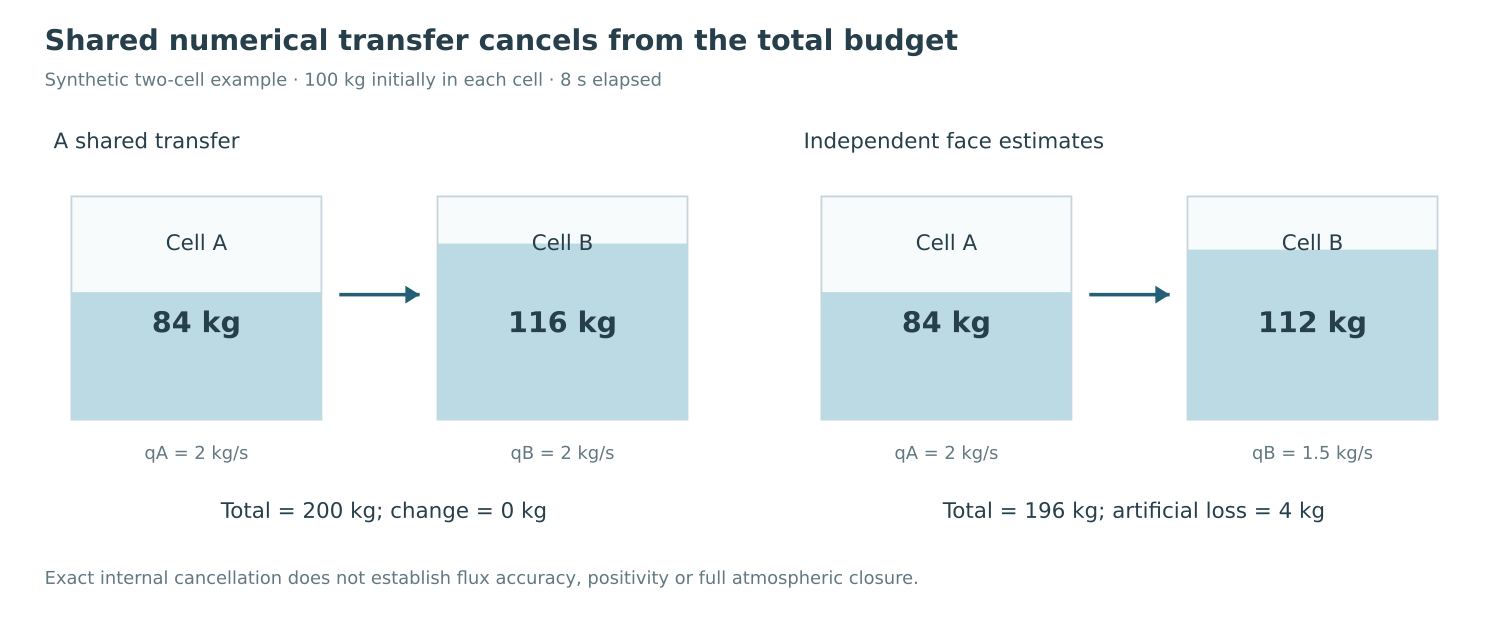
Synthetic two-cell accounting. The internal transfer cancels in the combined budget when both cells use the same value. An intentionally inconsistent interface reveals artificial mass loss or gain. Conservation of this toy quantity does not establish positivity, atmospheric closure or forecast skill.
Decomposition can reduce local approximation difficulty while introducing costs at interfaces and weakening the information available to each subproblem. Hu et al. (2022) formalise this conditional character for XPINNs: simpler local solution structure can favour decomposition, while splitting a fixed sample budget can counteract that benefit. FBPINNs address multiscale approximation through overlapping local networks and local normalisation, with their experiments also showing the importance of training schedules. Multilevel architectures subsequently add representations that communicate across larger portions of the domain. These studies support a comparison of locality, overlap and coarse communication; they do not supply a universal ordering of decomposed and global networks. For Caribbean moisture inference, partition size should therefore be related to observational support and transport scales, then varied within a prespecified comparison. Improved optimisation, reduced cost and improved recovery of withheld atmospheric structure are separate possible outcomes and should be measured separately. [94; 60; 26]
The D-LEGOS coupling proposition is conditional. A physically specified exchange may improve retrospective reconstruction where sparse observations and heterogeneous terrain make one global representation difficult to fit. That hypothesis may fail when observational constraints are too weak, when the equations omit dominant processes or when a simple operator model already captures the needed relationships. A doctoral contribution can identify those failure conditions. It should not depend on demonstrating that decomposition is universally superior.
7.3 Reconstruction in a space-time window
Retrospective reconstruction deserves its own statistical formulation. Let x₀:_t denote the sequence of atmospheric states in a window and y₀:_t the observations available over that window. A filtering distribution estimates a state using information available up to its time; a smoothing distribution can also use later observations. Schematically,
Equation 4. Filtering and smoothing condition on different evidence
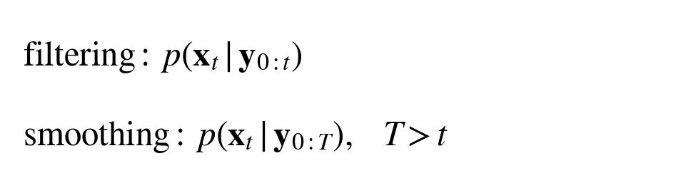
Editable notation: Filtering: p(x_t | y₀:t). Smoothing: p(x_t | y₀:T), T > t.
A filter uses evidence up to the state time. A smoother can use later observations. A forecast issued at an earlier time must exclude observations arriving after that issue time. The distinction is about information, not the direction of a neural-network call.
t — state time; time.
T — end of observation window; time.
p(·|·) — conditional distribution; density units depend on state.
The distinction is about the information set, rather than the direction in which a network is called. A model that uses observations from after an event to reconstruct conditions during it is performing retrospective inference. That can be scientifically valuable for understanding a poorly observed storm. Its result cannot be scored as an operational forecast issued before those observations existed. The forecasting literature reviewed above and the inverse reconstruction proposal must therefore be related through explicitly different evaluation protocols.
Explainer · The time machine has an information limit
A fictional time machine lets the investigator revisit yesterday after reading today’s instruments. A smoother does something mathematically similar with information: it conditions an earlier state on later observations. It does not reverse entropy or remove uncertainty about missing processes. To evaluate a forecast, move the information cutoff back to the issue time. To evaluate a reconstruction, retain the later information but withhold independent observations for checking. Calling both tasks “prediction” would conceal an advantage supplied by the observation window. [13; 32; 78]
Figure 5. Which observations is the model allowed to see?
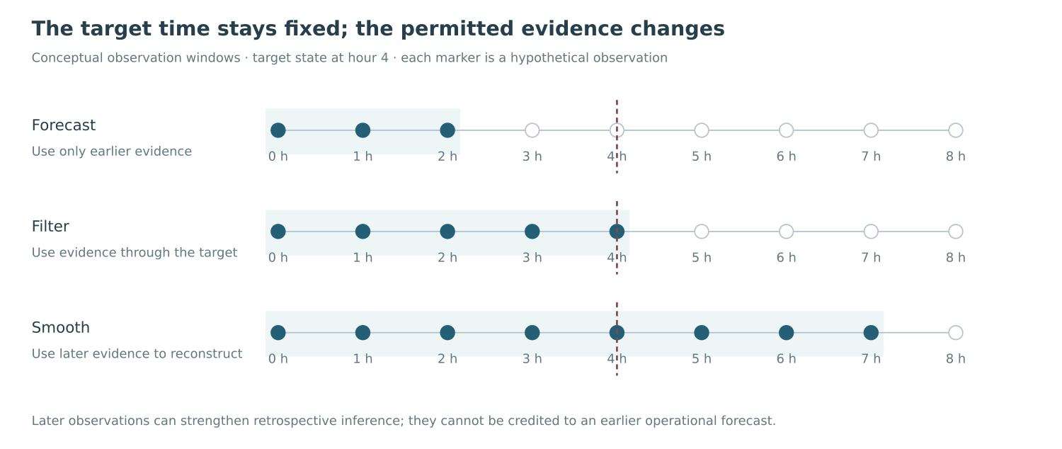
Conceptual observation windows. Forecasting, filtering and smoothing differ in their permitted evidence. Moving the cutoff does not change the historical observations; it changes which are available to the inference task.
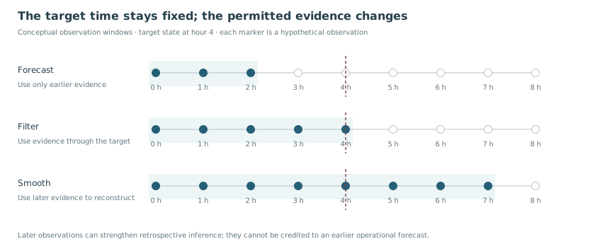
Bayesian language clarifies the problem even if the implementation uses deterministic optimisation. A schematic posterior combines a prior over admissible trajectories with the likelihood of the observations,
Equation 5. Posterior uncertainty combines evidence and prior assumptions

Editable notation: p(x₀:T | y₀:T) ∝ p(y₀:T | x₀:T) p(x₀:T).
The likelihood represents what the observations say about a trajectory. The prior represents assumptions before those observations are used. A physics penalty is not automatically a calibrated prior; its scale and model-error assumptions require justification.
x₀:T — trajectory; variable-dependent.
y₀:T — observations over the window; instrument-dependent.
∝ — proportional after normalisation; dimensionless relation.
Its practical value is to force attention to the observation operator, error model and prior assumptions. A squared-error penalty corresponds to a particular error assumption; it is not a neutral choice. Correlated retrieval errors and representativeness errors can make independent-error weighting overconfident. A physics residual may be interpreted as a regularising assumption, but it is not automatically a correctly specified probabilistic prior. Treating it as exact despite unresolved sources can exclude the real trajectory from the admissible set.
Observability is therefore central. Sparse measurements may constrain rainfall at a few sites while leaving vertical moisture structure or horizontal transport weakly identified. Several combinations of circulation and source terms can produce similar surface accumulations. Adding a smoothness penalty can select one solution, but does not show that the data identify it. The relevant literature on generative downscaling reinforces this point: unresolved fine scales can admit a distribution of plausible states [4; 1; 41; 53]. A single reconstruction should be described as a conditional estimate unless the uncertainty analysis supports a stronger claim.
This leads to an informative sequence of experiments. A synthetic system with known state, explicit observation geometry and controlled noise can establish whether the method recovers identifiable variables. Increasing sparsity, withholding vertical information and introducing source-term mismatch then expose where recovery fails. Those tests should precede claims about the unknown true state of a real historical event. A synthetic observing-system experiment is useful precisely because truth is available; it cannot demonstrate that the real atmosphere obeys the same error and closure assumptions.
Tasim and Sun reconstruct synthetic wind fields using weak divergence and near-ground regularisation, explicitly without solving the full Navier–Stokes system [75, section 6]. This provides a close comparator, while its synthetic setting leaves real-atmosphere validity open. The use of down-positive wind alongside altitude also makes coordinate-sign consistency an explicit verification item. D-LEGOS should distinguish its proposed coupled, moist atmospheric inference from this narrower task.
Classical variational and ensemble data assimilation form an essential comparison lineage as well. ERA5 exemplifies assimilation at atmospheric scale [44]. Weak-constraint variational assimilation, ensemble filtering and iterative smoothing provide direct comparators [78; 32; 13], discussed below.
7.4 Representation and interface uncertainty
A decomposed reconstruction introduces uncertainty in communication as well as in local state estimation. Overlapping blocks can reconcile inconsistent observations by averaging their fields, by exchanging boundary states, or by optimising common interface variables. These choices have different implications for conservation and uncertainty. Simple averaging may hide a disagreement that is scientifically informative. Independently sampled local generative outputs may be calibrated at each grid point while producing implausible cross-boundary structures. The joint field therefore needs evaluation beyond the distribution of isolated marginals.
This is a point of contact between domain-decomposition methods and probabilistic weather models. The former provide tools for local solution and communication [60; 25; 26; 69]; the latter motivate joint calibration, ensemble dependence and physically coherent spatial structure [28; 5]. Neither literature alone resolves the proposed combination. A useful D-LEGOS experiment would compare independent blocks, state-coupled blocks and flux-coupled blocks under the same observations, then assess how ensemble dependence and global budgets change. Such a comparison would isolate a contribution more clearly than a single comparison between the complete system and one weak baseline.
7.5 Assimilation and local neural fields describe related inverse problems
The distinction between assimilation and machine learning is not a distinction between using physics and using data. Geer places both within a common inverse-problem framework, emphasising uncertainty in observations, states and model parameters [35]. That framing prevents a neural reconstruction from claiming novelty simply because it combines observations with a physical model. The relevant comparison concerns what is inferred, which assumptions supply missing information and how the inference is approximated. The published correction changes the likelihood-to-objective factor [36]; the schematic objective below uses the conventional half-weighted quadratic form.
Trémolet distinguishes formulations that estimate model-error forcing, model bias or the four-dimensional atmospheric state [78]. The choice changes the control variable and the way imperfections in dynamics enter the reconstruction. This is directly relevant to D-LEGOS. A local field trained across a space-time window with physical residuals is conceptually closer to a weakly constrained state estimate than to a forecast model that simply evolves one initial condition. Its representation may differ substantially, but the inference principle has an established lineage.
Evensen's ensemble formulation represents uncertainty through a finite collection of states and covariance-based updates [32]. Bocquet and Sakov extend the comparison toward iterative smoothing and joint state–parameter estimation in controlled nonlinear systems [13]. These approaches make uncertainty representation and observability central rather than optional outputs of a generator. Their low-order or ensemble approximations bring limitations of their own. A finite ensemble can poorly represent high-dimensional dependence, while a variational estimate need not provide a complete posterior. Those limitations motivate comparison; they do not establish the superiority of a neural alternative.
Neural assimilation also has direct precedents beyond using a trained forecast model inside a conventional analysis. Fablet et al. (2021) jointly learn a dynamical representation and a variational solver, with numerical experiments on Lorenz-63 and Lorenz-96. Their work makes learned optimisation and the choice of dynamical prior part of the reconstruction problem itself. Neural operators address a related but distinct form of reuse: the Fourier neural operator learns mappings between function-valued inputs and outputs, while the physics-informed neural operator combines data with differential-equation residuals, including residual evaluation at a finer resolution than the training data. These precedents require the review to state which part of D-LEGOS is learned across cases and which part is fitted within a reconstruction window. A method trained to solve a family of inverse problems has different amortisation costs and generalisation requirements from one that optimises a new field for every event. [98; 95; 54]
A schematic weak-constraint objective clarifies the relationship:
Equation 6. Weak-constraint four-dimensional variational inference
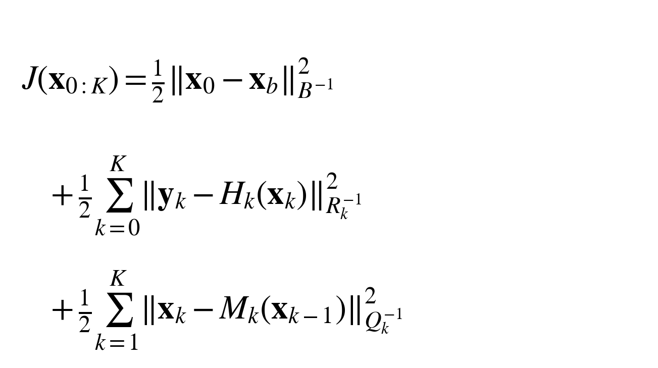
Editable notation: J = ½‖x₀−x_b‖²_B⁻¹ + ½Σ‖y_k−H_k(x_k)‖²_R_k⁻¹ + ½Σ‖x_k−M_k(x_k₋₁)‖²_Q_k⁻¹.
The three terms penalise departures from background, observations and imperfect model evolution. Covariances set their relative evidential weight. With correctly dimensioned covariances each quadratic term is dimensionless. Correlated errors require a joint formulation; the displayed sums assume the stated factorisation. The displayed quadratic form assumes fixed positive-definite covariances. Jointly estimated or state-dependent covariances require the normalised likelihood, including log-determinant terms, and stated priors.
B — background-error covariance; state units squared.
R_k — observation-error covariance; observed units squared.
Q_k — model-error covariance; state units squared.
M_k — evolution map; state to state.
x_b — background state; variable-dependent.
Here the background term constrains the initial state, the observation terms measure model–observation discrepancies with covariance R, and the model terms measure departures from a specified evolution map with covariance Q. B describes background uncertainty. The notation is schematic: temporally correlated errors require a joint covariance rather than the independent sum displayed. A neural field changes the parameterisation of the state sequence; a physics residual can replace or augment part of the evolution discrepancy. Neither substitution removes the need to define the uncertainties and approximation regime. Here ‖v‖²_C⁻¹ = v^TC⁻¹v, with fixed positive-definite covariance matrices in this schematic state-estimation objective. If uncertainty parameters or state-dependent covariances are estimated jointly, their normalised likelihood terms and stated priors must be retained. In consistently scaled coordinates, a Gaussian model-error contribution then includes both ½e^TQ⁻¹e and ½ log det Q, up to constants; the corresponding normalisation applies to other estimated covariances. Alternatively, covariances can be independently calibrated and fixed before state estimation.
For local representations, an interface contribution can be added to this objective. If an edge denotes a shared transfer, the outward transfers for the two adjacent control volumes must use opposite orientations and consistent measures. That is an implementation condition. The scientific question is whether this coupling improves the inferred interior state and physical diagnostics at withheld locations and times. Minimising an interface term on the same sampled faces used for training is not sufficient evidence of that improvement.
Table 5 Closest inference and decomposition lineages
| Formulation | Unknowns and discrepancy | Communication and uncertainty | What remains to test |
|---|---|---|---|
| Weak-constraint 4D-Var [78] | Initial state plus model forcing or bias, or the four-dimensional state itself. | Dynamical evolution links times; background, observation and model-error terms constrain the estimate. | A neural parameterisation must improve a specified outcome beyond renaming this inverse problem. |
| Ensemble Kalman filter [32] | State ensemble updated through approximate covariance relationships. | Sequential updates represent finite-ensemble uncertainty; later observations require smoothing. | Match the observation window and distinguish ensemble approximation error from model error. |
| Iterative ensemble smoother [13] | Joint state and parameter estimation in the examined nonlinear systems. | Window-based inference with ensemble approximations and iterative updates. | Real-atmosphere transfer and state–closure identifiability are separate questions. |
| FBPINNs and multilevel FBPINNs [60; 26] | Local neural fields for specified differential-equation problems. | Overlapping support and multilevel correction improve communication in the evaluated benchmarks. | Atmospheric moisture inference with uncertain observations is not established by solver scaling alone. |
| Parallel cPINN and XPINN [69] | Local solution representations with conservative or more flexible decompositions. | Interface conditions and parallel schedules define the mathematical and computational exchange. | The physically relevant atmospheric flux and coordinate measure still need definition. |
| Conservative PINNs [92] | Local neural fields for conservation-law subdomains. | Shared-interface flux mismatches enter the inspected implementation as penalties. | A conservative physical form is distinct from exact algebraic flux cancellation. |
| Extended PINNs [93] | Neural approximations over decomposed space–time domains. | Interface losses and local representations define exchange. | Local space–time decomposition itself is established prior art. |
| Learned variational assimilation [98] | Jointly learned dynamical representations and variational inference solvers. | Observation and dynamical information constrain trajectories; evaluated on Lorenz systems. | Regional atmospheric transfer and independent moisture reconstruction remain separate tests. |
| D-LEGOS restricted proposal | Local resolved wind, temperature and humidity fields with bounded tendencies. | Specified shared moisture transfer plus observation, background and discrepancy information. | Does exchange improve withheld state recovery, budgets and uncertainty under driver bias and sparsity? |
The existing decomposition studies identify a related computational distinction. FBPINNs use local overlapping networks and local normalisation [60]. Their multilevel extension improves communication across many subdomains in the examined differential-equation benchmarks [26]. Parallel cPINN and XPINN formulations compare conservative spatial exchanges with more flexible decompositions in space and time [69]. They establish that locality, overlap, coarse communication and parallel execution are already substantive numerical design choices. The proposed atmospheric contribution must therefore concern a specified combination of these choices under a defined observation and moisture-budget problem.
Read together, assimilation and decomposition expose two distinct explanations of improvement. A local representation may make optimisation easier without adding observational information. Alternatively, a physical exchange can restrict an otherwise underdetermined state more appropriately. A careful comparison separates those explanations by matching data and computational effort, and by examining state recovery and uncertainty as well as training loss. The literature supports that interaction question; it does not support treating an interacting graph or a space-time block as intrinsically novel.
8 The contribution supported by the synthesis
8.1 A question about moisture inference under incomplete observations
The reviewed literature establishes plausible components rather than an unoccupied methodological category. Regional climate studies define a physical environment in which moisture transport, stability and terrain matter. Downscaling studies show how coarse-driver error and unresolved fine scales complicate statistical refinement. Physical learning studies distinguish imposed consistency from independently demonstrated skill. Assimilation and decomposition supply close precedents for state estimation and local numerical representation. The unresolved question developed here lies at their intersection: how much benefit physically specified local exchange provides when the observations and large-scale atmospheric reference are both incomplete or uncertain.
The primary contribution sought from D-LEGOS is therefore knowledge about reconstructing moisture transport and rainfall-relevant atmospheric structure over island domains. The architecture is a means of testing that question. A useful answer would identify conditions under which physical exchange improves inference, conditions under which it transmits a biased background, and conditions under which observations cannot distinguish competing states. This remains a proposed contribution; it is not an empirical result of the review or a claim that no earlier study has examined any part of the problem.
The proposed contribution is a controlled account of when physically specified local exchanges improve moisture inference over island domains, relative to the existing assimilation and decomposition lineages. The principal atmospheric experiment compares uncoupled, state-coupled and flux-coupled representations under the same observation window, masks, boundary information and documented treatment of unresolved tendencies. Its endpoint is recovery of withheld moisture-related quantities and independently computed transport or budget diagnostics at the declared mesoscale. A separate precipitation-allocation experiment addresses H1 by varying coarse-driver bias while testing aggregation constraints. That companion experiment does not make precipitation a prognostic variable in the restricted hydrostatic reconstruction. Together, the experiments can identify circumstances in which an exact relationship transmits useful information or propagates a biased reference. They can also distinguish better optimisation from a better-constrained inverse problem. The contribution remains conditional and proposed: space–time partitioning, neural variational inference and physical penalties already have established predecessors, while the regional interaction of exchange, observational geometry and driver uncertainty requires empirical testing. [92; 93; 94; 26; 54; 98]
Three levels of outcome are kept separate. Numerical verification establishes whether the implemented aggregation and exchange conditions actually hold. Reconstruction evaluation establishes whether the field is better supported by withheld observations and independently computed diagnostics. Physical interpretation examines what the result establishes about transport, storage and the uncertainty of the inferred process. Only the latter two can supply the intended scientific answer; a constraint satisfied by construction belongs to the first level.
8.2 Falsifiable hypotheses
H1. A companion precipitation-allocation experiment tests the interaction between aggregation constraints and coarse-driver bias. Under sufficiently accurate coarse forcing, exact aggregation is hypothesised to improve or preserve independently evaluated precipitation allocation relative to a matched unconstrained learner. Under systematically biased forcing, that advantage is hypothesised to diminish and may reverse. The scientific outcome is the change in withheld observational skill across documented bias regimes. A model whose aggregation error is zero but whose independent error worsens does not support the beneficial part of the hypothesis. The bias level at which performance changes is to be estimated from the comparison, not assumed as a universal threshold.
H2. The principal atmospheric reconstruction experiment tests coupling between local representations. With matched observations and comparable model capacity and computational effort, flux-aware coupling is hypothesised to lower withheld moisture-transport error relative to state-only and uncoupled representations as observation coverage becomes sparse. In a controlled observing-system experiment, vector vapour transport and moisture-flux convergence can be compared with the known reference state. In real events, withheld observed quantities and independently assembled budget terms provide a narrower test; an unobserved transport field is not labelled validated merely because it agrees with the background. The observation masks and sparsity levels must be fixed before evaluation, rather than selected after favourable results appear. Exact fitted interface agreement can coexist with a rejected hypothesis when incorrect closures or boundary information worsen interior recovery.
H3 concerns uncertainty and observation geometry. Explicit representation of background and model discrepancy is hypothesised to improve probabilistic reconstruction relative to a matched uncertainty model that treats those inputs as fixed. Both approaches use the same observation windows and prespecified masks. Model selection, probability calibration and final evaluation use separate event or time blocks; calibration parameters are frozen before scores and coverage are computed on the final test blocks. Its outcomes are a lower proper score for defined withheld quantities, coverage closer to the declared nominal level, and credible joint spatial dependence. A deterministic comparator requires a separately calibrated probabilistic extension before distributional scores are compared. Wider intervals alone do not support the hypothesis. Incorrect discrepancy structure can worsen sharpness, calibration or dependence, so an uncertainty-aware model can fail even when its samples look plausible.
8.3 Boundaries of the novelty claim
These hypotheses distinguish the proposed investigation from a generic claim that combining physics and AI improves climate prediction. The closest comparisons remain hard-constrained downscaling, weak-constraint assimilation, multilevel local neural solvers and hybrid dynamical-core models [40; 78; 26; 49]. The specific research difference concerns the controlled interaction of observation geometry, biased large-scale information and local physical exchange in a regional moisture-inference problem. A claim of an entirely new inference principle would exceed the evidence reviewed here.
Historical reconstruction is the first scientific endpoint. A forward rollout from a reconstructed state asks a secondary question about the usefulness and dynamical adequacy of that state. Long-run climate statistics and responses to altered forcing are further claims requiring separate evidence. This hierarchy makes the Caribbean climate-physics motivation concrete without requiring a successful historical reconstruction to establish future climate fidelity. It also allows a negative result to be informative: a simpler representation may remain preferable, or coupling may be useful only when the observation network leaves a particular transport structure unresolved.
9 What the comparison literature requires of evidence
9.1 The target determines the relevant comparator
The literature does not support one universal leaderboard for downscalers, reconstructors and climate emulators. Van der Meer's perfect and imperfect frameworks demonstrate why changing the driver changes the inference problem [79]. Harris's stochastic rainfall study shows why a conditional distribution cannot be judged solely through the error of its mean [41]. Trémolet's control formulations show that changing the treatment of model error changes the state-estimation problem [78]. These distinctions require comparisons to be organised around the target and information set before architectural performance is interpreted.
For a reconstruction question, the critical reference points are the background state, a strong statistical interpolation or smoothing method, a nondecomposed representation and an assimilation formulation with a comparable observation window. Decomposed models then isolate what communication contributes. Seasonal and terrain-aware baselines remain particularly important for precipitation allocation because broad recurring spatial structure can explain a substantial part of that task without a fully coupled atmosphere. A comparison with an intentionally weak interpolator would leave that alternative explanation unresolved.
A complete system comparison and a mechanism comparison answer different questions. The first may allow each approach its best practical configuration. The second holds relevant resources and information sufficiently close to isolate the chosen design. Both can be useful, but an apparent benefit caused by additional parameters, observations or tuning is not clean evidence for the physical interface. The optimisation studies reinforce this distinction: physical regularisation can change conditioning and training difficulty even when the represented solution class is adequate [50; 81].
9.2 Verification across space time and physical regime
A split between neighbouring pixels does not establish transfer between genuinely different atmospheric situations. Spatially and temporally dependent observations can make a held-out point resemble the training set closely. The relevant unit of separation depends on the claim: contiguous windows for temporal reconstruction, complete events for event transfer, and geographically meaningful domains for island transfer. The observed distinction between regional mechanisms and product support makes a leave-island-out experiment different from random point withholding on an already represented island [47; 17; 20].
Transfer to a changed climate is more demanding than interpolation within a historical record. Hernanz and colleagues examine limitations of statistical downscaling under transfer and extrapolation [43], while Baño-Medina and colleagues study transferability of regional emulators [11]. Clarke's changing early-season rainfall associations provide a regionally relevant reason to question stationary relationships [22]. These studies do not establish one correction that resolves all distribution change. They show why a model should be evaluated against the particular regime change for which usefulness is claimed.
For a historical event study, a demanding case can expose mechanism and failure, but cannot by itself establish the frequency or distribution of those failures. Conversely, an aggregate score across many ordinary cases can conceal a physically important event failure. The two forms of evidence are complementary: case analysis tests whether the inferred transport and storage are physically interpretable, while broader evaluation tests how often and where that interpretation remains useful.
9.3 Predictive skill and physical consistency can disagree
The nowcasting comparison of Das and colleagues provides a concrete example [23]. NowcastNet improves heavy-rainfall detection against the evaluated numerical and simpler comparators, while the paper retains a caveat about aggregate precipitation at longer leads. This is precisely the kind of result that a single score could obscure. A model can improve one aspect of a rainfall event and worsen another quantity important to water accounting. It would be inappropriate to transfer either the reported advantage or its magnitude directly to a different region, horizon or reconstruction task.
Hard-constrained downscaling supplies the converse warning [40]. Exact agreement with a prescribed total proves a selected relationship within the implementation. It does not prove that the total or the spatial allocation is correct. A rigorous interpretation therefore considers independent observation errors and physical diagnostics together. Where independent measurements do not exist, the conclusion is limited to consistency and reference-system fidelity rather than an observationally validated atmospheric state.
The diagnostics themselves can share assumptions with the model. Recomputing a residual at the same training points with the same differentiation operator is partly a test of the fitted objective. Independent locations, alternative conservative diagnostics and sensitivity to discretisation provide a stronger assessment of the field. Moisture budgets require storage and boundary terms at the stated support; sharp rainfall images and pointwise temperature agreement do not supply those terms. The physical and observation operators define what a diagnostic can establish.
Figure 6. A forecast can improve on one metric and worsen on another
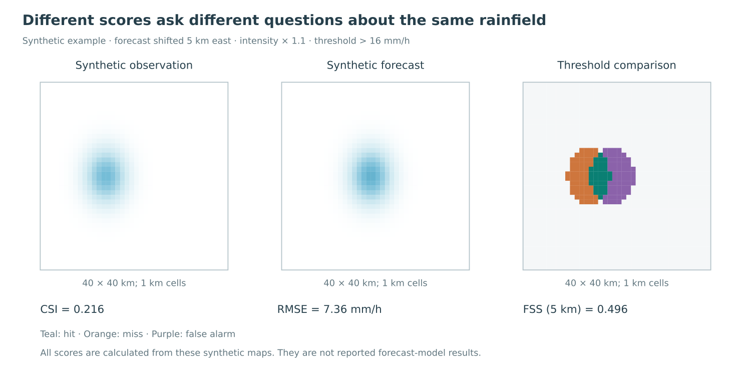
Computed metrics for synthetic fields. Change displacement, intensity, threshold and neighbourhood size. CSI, RMSE and FSS measure different properties; changing the neighbourhood changes the verification question. The values are not published model scores. [111]
9.4 Uncertainty and computational usefulness
The generative and ensemble literatures show why uncertainty cannot be reduced to visual variety [28; 41; 5]. Marginal calibration does not establish realistic cross-variable or spatial dependence. High coverage can be obtained by an uninformatively broad distribution, while sharp samples can be systematically overconfident. A useful probabilistic comparison therefore preserves both informativeness and calibration for defined variables, and examines whether physically relevant joint structures survive conditioning on sparse observations.
Uncertainty in a reconstruction also has different sources: measurement and representation error, uncertainty of the initial or background state, model discrepancy and non-identifiability. An ensemble of network fits does not automatically represent all of them. Assimilation supplies established ways to organise these distinctions [32; 13], while generative downscaling supplies tools for unresolved conditional variation [4; 1; 53]. Their combination is potentially useful only if the roles of those uncertainties remain explicit.
Computational claims require an equally explicit boundary. A trained network's inference time excludes the cost of learning its weights, searching hyperparameters, preparing observations or producing ensembles. A model that reconstructs one field and a model that evolves a coupled atmosphere provide different outputs. Comparing their runtimes without the task definition can create an apparent speed advantage that does not answer the scientific question. The relevant contribution is a useful trade-off between supported information, uncertainty and total effort at the declared scale.
The research gap should be expressed as a falsifiable comparison rather than a general promise of physically informed prediction. A suitable question is whether conservative exchange between regional space-time modules improves prespecified moisture-transport reconstruction, budget diagnostics and uncertainty estimates under matched observations and computational resources. H1 addresses rainfall allocation in a separate companion experiment. Global benchmarking practice offers useful infrastructure, while Caribbean product comparisons show why observation independence and accumulation scale require additional attention. The proposed test should withhold complete storms, years or locations according to the intended generalization claim. It should report continuous error, threshold-event skill, probabilistic calibration and spatial displacement separately, with uncertainty estimated at a unit that respects dependence. A model that improves water accounting while failing to improve storm timing would yield a meaningful result. The interpretation should identify that trade-off rather than convert several outcomes into one unsupported label of overall superiority. [109; 20; 110; 111]
10 Synthesis
The literature supports a physically motivated investigation of local atmospheric reconstruction in the Caribbean, but places clear limits on the claims that investigation can make. Regional climate studies establish why circulation, moisture transport, stability and terrain belong in the same physical account. Observational studies show that the fields used to examine those processes are themselves uncertain reconstructions. Downscaling and emulation provide effective ways to refine information, while assimilation and domain decomposition supply established principles for combining observations, imperfect dynamics and local representation.
The main unresolved issue is not whether a model can include physical equations or generate a detailed rainfall map. It is whether the chosen physical exchange between local learned fields provides independently useful information about a partially observed atmospheric state. The answer depends on the quality of the driver, the observation geometry, the treatment of unresolved processes and the validity of the approximation regime. The D-LEGOS question makes those dependencies part of the proposed contribution.
A positive result would establish a regime in which the reconstructed transport or rainfall-relevant structure is better supported than under the closest alternatives. A negative result could identify a driver bias that hard constraints propagate, an unidentifiable vertical structure, or a scale at which a simpler model remains preferable. Either can advance the intended physical understanding if the information set and comparison are explicit. Forecasting and climate-response applications then follow as separately justified extensions, supported by evidence appropriate to their own claims.
Appendix A. Review method and source coverage
This is a critical thematic literature review, updated on 24 October 2026 from the author’s revision 06 dated 15 October 2026. Its central question remains retrospective reconstruction of rainfall-relevant moisture transport under incomplete observations and uncertain large-scale forcing. The selection follows the closest physical, statistical and numerical lineages; it is not presented as an exhaustive systematic review or meta-analysis.
The existing register contains 275 records, including stored copies and records of different access status; these are not treated as 275 unique, fully appraised studies. The connected Anara collection contains 173 document items. A current first-page retrieval was attempted for every item: 127 returned readable passages and 46 returned no readable text. First-page screening is distinguished from full-text appraisal. Targeted Anara searches and page reads were used for regional circulation, the Jamaica rainfall example, hard-constrained downscaling and selected physical-learning methods. Publication pages, institutional documentation, author manuscripts and the supplied PDF supplied additional evidence.
All 88 entries in revision 06’s bibliography were checked for bibliographic identity against publication records, DOI metadata, arXiv records or the identified stored technical report. The resulting evidence record distinguishes metadata checks, abstract-level evidence and full-text or selected-section reading. New sources were added for direct domain-decomposition precedents, uncertainty scores, precipitation verification, generative downscaling and 2026 hybrid precipitation studies. An inaccessible paper is not assigned an empirical finding from its title. DOI existence alone is not a claim-support check.
Searches combined project terms such as “Caribbean moisture transport reconstruction”, “Jamaica CHIRPS gauge precipitation validation”, “early season warming Caribbean predictability”, “downscaling hard constraint biased coarse field”, “Accounting for an imperfect model in 4D-Var”, and targeted model and paper titles. The evidence table records the access depth and the exact supported claim where a new focused appraisal was performed. Existing source interpretations were retained only within the bounded argument of the revised review. Inherited synthesis with a refreshed metadata check is explicitly marked in the evidence explorer.
The update reconciles identifiable publication versions where verified, including the journal versions of selected physics-informed methods and the climate-emulator review. Known corrections to the small-island rainfall study and Geer’s inverse-problem paper remain part of the bibliography. Publisher and registry update metadata were inspected when available; this is not a certification that every possible correction or retraction notice has been exhaustively located. The unresolved abstract–figure attribution in the supplied nowcasting paper is retained as a numerical-reporting check rather than converted into a new quantitative claim. [23; 35; 36; 70; 71]
Appendix B. Reading the scientific illustrations
All newly drawn scientific illustrations are explanatory constructions made for this review. The metric playground evaluates synthetic arrays generated by stated controls. The flux widget applies a discrete accounting identity to a closed two-cell system. The resolution widget constructs nonnegative fields with a prescribed equal-area mean. The time-window figure identifies permitted observations. None reports a newly trained D-LEGOS model, measured Caribbean forecast skill, or a reproduction of a published benchmark.
The science-fiction vignettes are fictional thought experiments written to explain information and conservation limits. They are not autobiographical anecdotes, quotations attributed to Richard Feynman, or evidence for the research findings. Their role is to make the reasoning accessible while leaving the academic argument intact.
Data, code and author statements
This review reports no new human-participant study and no new atmospheric model benchmark. Its original contribution is critical synthesis and a proposed research question. The interactive calculations and figure-generating code accompany the paper. Source papers remain credited to their authors and are linked rather than redistributed. Adrian Dunkley retains responsibility for the scientific interpretation and final manuscript; this version is for author and supervisory review. No journal acceptance, institutional endorsement or completed doctoral validation is implied.
References
[1] Addison, H.; Kendon, E.; Ravuri, S.; Aitchison, L.; Watson, P. A. (2024). Machine learning emulation of precipitation from km-scale UK regional climate simulations using a diffusion model. arXiv:2407.14158v2 [preprint]. https://arxiv.org/abs/2407.14158v2
[2] Afshari, A.; Vogel, J.; Chockalingam, G. (2023). Statistical Downscaling of SEVIRI Land Surface Temperature to WRF Near-Surface Air Temperature Using a Deep Learning Model. Remote Sensing, 15(18), 4447. https://doi.org/10.3390/rs15184447
[3] Agrawal, S.; Hassen, M. A.; Brempong, E. A.; Babenko, B.; Zyda, F.; Graham, O.; Li, D.; Merchant, S.; Potes, S. H.; Russell, T.; Cheresnick, D.; Kakkirala, A. P.; Rasp, S.; Hassidim, A.; Matias, Y.; Kalchbrenner, N.; Gupta, P.; Hickey, J.; Bell, A. (2025). An Operational Deep Learning System for Satellite-Based High-Resolution Global Nowcasting. arXiv:2510.13050v1 [preprint]. https://arxiv.org/abs/2510.13050v1
[4] Aich, M.; Hess, P.; Pan, B.; Bathiany, S.; Huang, Y.; Boers, N. (2024). Conditional diffusion models for downscaling and bias correction of Earth system model precipitation. arXiv:2404.14416v2 [preprint]. https://arxiv.org/abs/2404.14416v2
[5] Alet, F.; Price, I.; El-Kadi, A.; Masters, D.; Markou, S.; Andersson, T. R.; Stott, J.; Lam, R.; Willson, M.; Sanchez-Gonzalez, A.; Battaglia, P. (2025). Skillful joint probabilistic weather forecasting from marginals. arXiv:2506.10772v1 [preprint]. https://arxiv.org/abs/2506.10772v1
[6] Allen, A.; Markou, S.; Tebbutt, W.; Requeima, J.; Bruinsma, W. P.; Andersson, T. R.; Herzog, M.; Lane, N. D.; Chantry, M.; Hosking, J. S.; Turner, R. E. (2025). End-to-end data-driven weather prediction. Nature, 641(8065), 1172-1179. https://doi.org/10.1038/s41586-025-08897-0
[7] Andrychowicz, M.; Espeholt, L.; Li, D.; Merchant, S.; Merose, A.; Zyda, F.; Agrawal, S.; Kalchbrenner, N. (2023). Deep Learning for Day Forecasts from Sparse Observations. arXiv:2306.06079v3 [preprint]. https://arxiv.org/abs/2306.06079v3
[8] Avalon Cullen, C.; Al Suhili, R. (2023). Assessing Rainfall Variability in Jamaica Using CHIRPS: Techniques and Measures for Persistence, Long and Short-Term Trends. Geographies, 3(2), 375-397. https://doi.org/10.3390/geographies3020020
[9] Balaguru, K.; Foltz, G. R.; Leung, L. R. (2018). Increasing Magnitude of Hurricane Rapid Intensification in the Central and Eastern Tropical Atlantic. Geophysical Research Letters, 45(9), 4238-4247. https://doi.org/10.1029/2018gl077597
[10] Baño-Medina, J.; Manzanas, R.; Gutiérrez, J. M. (2020). Configuration and intercomparison of deep learning neural models for statistical downscaling. Geoscientific Model Development, 13(4), 2109-2124. https://doi.org/10.5194/gmd-13-2109-2020
[11] Baño-Medina, J.; Iturbide, M.; Fernández, J.; Gutiérrez, J. M. (2024). Transferability and Explainability of Deep Learning Emulators for Regional Climate Model Projections: Perspectives for Future Applications. Artificial Intelligence for the Earth Systems, 3(4). https://doi.org/10.1175/aies-d-23-0099.1
[12] Bi, K.; Xie, L.; Zhang, H.; Chen, X.; Gu, X.; Tian, Q. (2023). Accurate medium-range global weather forecasting with 3D neural networks. Nature, 619(7970), 533-538. https://doi.org/10.1038/s41586-023-06185-3
[13] Bocquet, M.; Sakov, P. (2013). Joint state and parameter estimation with an iterative ensemble Kalman smoother. Nonlinear Processes in Geophysics, 20(5), 803-818. https://doi.org/10.5194/npg-20-803-2013
[14] Bodnar, C.; Bruinsma, W. P.; Lucic, A.; Stanley, M.; Allen, A.; Brandstetter, J.; Garvan, P.; Riechert, M.; Weyn, J. A.; Dong, H.; Gupta, J. K.; Thambiratnam, K.; Archibald, A. T.; Wu, C. C.; Heider, E.; Welling, M.; Turner, R. E.; Perdikaris, P. (2025). A foundation model for the Earth system. Nature, 641(8065), 1180-1187. https://doi.org/10.1038/s41586-025-09005-y
[15] Brown, C. F.; Kazmierski, M. R.; Pasquarella, V. J.; Rucklidge, W. J.; Samsikova, M.; Zhang, C.; Shelhamer, E.; Lahera, E.; Wiles, O.; Ilyushchenko, S.; Gorelick, N.; Zhang, L. L.; Alj, S.; Schechter, E.; Askay, S.; Guinan, O.; Moore, R.; Boukouvalas, A.; Kohli, P. (2025). AlphaEarth Foundations: An embedding field model for accurate and efficient global mapping from sparse label data. arXiv:2507.22291v2 [preprint]. https://arxiv.org/abs/2507.22291v2
[16] Campbell, J. D.; Taylor, M. A.; Stephenson, T. S.; Watson, R. A.; Whyte, F. S. (2011). Future climate of the Caribbean from a regional climate model. International Journal of Climatology, 31(12), 1866-1878. https://doi.org/10.1002/joc.2200
[17] Campbell, J. D.; Taylor, M. A.; Bezanilla-Morlot, A.; Stephenson, T. S.; Centella-Artola, A.; Clarke, L. A.; Stephenson, K. A. (2021). Generating Projections for the Caribbean at 1.5, 2.0 and 2.5 °C from a High-Resolution Ensemble. Atmosphere, 12(3), 328. https://doi.org/10.3390/atmos12030328
[18] Centella, A.; Bezanilla, A.; Leslie, K. R. (2008). A Study of the Uncertainty in Future Caribbean Climate Using the PRECIS Regional Climate Model. Technical report, Caribbean Community Climate Change Centre. Technical report retained in the author’s reference collection.
[19] Centella-Artola, A.; Taylor, M. A.; Bezanilla-Morlot, A.; Martinez-Castro, D.; Campbell, J. D.; Stephenson, T. S.; Vichot, A. (2015). Assessing the effect of domain size over the Caribbean region using the PRECIS regional climate model. Climate Dynamics, 44(7-8), 1901-1918. https://doi.org/10.1007/s00382-014-2272-8
[20] Centella-Artola, A.; Bezanilla-Morlot, A.; Taylor, M. A.; Herrera, D. A.; Martinez-Castro, D.; Gouirand, I.; Sierra-Lorenzo, M.; Vichot-Llano, A.; Stephenson, T.; Fonseca, C.; Campbell, J.; Alpizar, M. (2020). Evaluation of Sixteen Gridded Precipitation Datasets over the Caribbean Region Using Gauge Observations. Atmosphere, 11(12), 1334. https://doi.org/10.3390/atmos11121334
[21] Chen, L.; Zhong, X.; Zhang, F.; Cheng, Y.; Xu, Y.; Qi, Y.; Li, H. (2023). FuXi: a cascade machine learning forecasting system for 15-day global weather forecast. npj Climate and Atmospheric Science, 6(1), 190. https://doi.org/10.1038/s41612-023-00512-1
[22] Clarke, L. A.; Jones, J. J.; Taylor, M. A.; Williams, M. S. M.; Edwards, T.; Stephenson, T. S. (2026). Breaking the link: warming disrupts early-season rainfall predictability in the Caribbean. npj Climate and Atmospheric Science, 9(1), 52. https://doi.org/10.1038/s41612-026-01325-8
[23] Das, P.; Posch, A.; Barber, N.; Hicks, M.; Duffy, K.; Vandal, T.; Singh, D.; Werkhoven, K. v.; Ganguly, A. R. (2024). Hybrid physics-AI outperforms numerical weather prediction for extreme precipitation nowcasting. npj Climate and Atmospheric Science, 7(1), 282. https://doi.org/10.1038/s41612-024-00834-8
[24] Dheeshjith, S.; Subel, A.; Adcroft, A.; Busecke, J.; Fernandez-Granda, C.; Gupta, S.; Zanna, L. (2024). Samudra: An AI Global Ocean Emulator for Climate. arXiv:2412.03795v4 [preprint]. https://arxiv.org/abs/2412.03795v4
[25] Dolean, V.; Heinlein, A.; Mishra, S.; Moseley, B. (2022). Finite basis physics-informed neural networks as a Schwarz domain decomposition method. arXiv:2211.05560v2 [preprint]. https://arxiv.org/abs/2211.05560v2
[26] Victorita Dolean; Alexander Heinlein; Siddhartha Mishra; Ben Moseley (2024). Multilevel domain decomposition-based architectures for physics-informed neural networks. Computer Methods in Applied Mechanics and Engineering 429, 117116. https://doi.org/10.1016/j.cma.2024.117116
[27] Doury, A.; Somot, S.; Gadat, S.; Ribes, A.; Corre, L. (2023). Regional climate model emulator based on deep learning: concept and first evaluation of a novel hybrid downscaling approach. Climate Dynamics, 60(5-6), 1751-1779. https://doi.org/10.1007/s00382-022-06343-9
[28] Du, J.; Sadeghi Tabas, S.; Wang, J.; Levit, J. (2025). Understanding Similarities and Differences Between Data-Driven AI Model-Based and Physics Model-Based Ensemble Forecasts. NCEP Office Note 523, NOAA. https://doi.org/10.25923/4pc4-3t39
[29] Dullaart, J. C. M.; de Vries, H.; Bloemendaal, N.; Aerts, J. C. J. H.; Muis, S. (2024). Improving our understanding of future tropical cyclone intensities in the Caribbean using a high-resolution regional climate model. Scientific Reports, 14(1), 6108. https://doi.org/10.1038/s41598-023-49685-y
[30] Duncan, J. P. C.; Wu, E.; Golaz, J. C.; Caldwell, P. M.; Watt‐Meyer, O.; Clark, S. K.; McGibbon, J.; Dresdner, G.; Kashinath, K.; Bonev, B.; Pritchard, M. S.; Bretherton, C. S. (2024). Application of the AI2 Climate Emulator to E3SMv2's Global Atmosphere Model, With a Focus on Precipitation Fidelity. Journal of Geophysical Research: Machine Learning and Computation, 1(3), e2024JH000136. https://doi.org/10.1029/2024jh000136
[31] Duncan, J. P. C.; Wu, E.; Dheeshjith, S.; Subel, A.; Arcomano, T.; Clark, S. K.; Henn, B.; Kwa, A.; McGibbon, J.; Perkins, W. A.; Gregory, W.; Fernandez-Granda, C.; Busecke, J.; Watt-Meyer, O.; Hurlin, W. J.; Adcroft, A.; Zanna, L.; Bretherton, C. (2025). SamudrACE: Fast and Accurate Coupled Climate Modeling with 3D Ocean and Atmosphere Emulators. arXiv:2509.12490v1 [preprint]. https://arxiv.org/abs/2509.12490v1
[32] Evensen, G. (2003). The Ensemble Kalman Filter: theoretical formulation and practical implementation. Ocean Dynamics, 53(4), 343-367. https://doi.org/10.1007/s10236-003-0036-9
[33] Funk, C.; Peterson, P.; Landsfeld, M.; Pedreros, D.; Verdin, J.; Shukla, S.; Husak, G.; Rowland, J.; Harrison, L.; Hoell, A.; Michaelsen, J. (2015). The climate hazards infrared precipitation with stations—a new environmental record for monitoring extremes. Scientific Data, 2(1), 150066. https://doi.org/10.1038/sdata.2015.66
[34] García-Franco, J. L.; Chadwick, R.; Gray, L. J.; Osprey, S.; Adams, D. K. (2023). Revisiting mechanisms of the Mesoamerican Midsummer drought. Climate Dynamics, 60(1-2), 549-569. https://doi.org/10.1007/s00382-022-06338-6
[35] Geer, A. J. (2021). Learning earth system models from observations: machine learning or data assimilation?. Philosophical Transactions of the Royal Society A: Mathematical, Physical and Engineering Sciences, 379(2194), 20200089. https://doi.org/10.1098/rsta.2020.0089
[36] Geer, A. J. (2022). Correction to ‘Learning earth system models from observations: machine learning or data assimilation?’. Philosophical Transactions of the Royal Society A: Mathematical, Physical and Engineering Sciences, 380(2220), 20220004. https://doi.org/10.1098/rsta.2022.0004
[37] Giannini, A.; Kushnir, Y.; Cane, M. A. (2000). Interannual Variability of Caribbean Rainfall, ENSO, and the Atlantic Ocean. Journal of Climate, 13(2), 297-311. https://doi.org/10.1175/1520-0442(2000)013<0297:ivocre>2.0.co;2
[38] Guan, H.; Arcomano, T.; Chattopadhyay, A.; Maulik, R. (2024). LUCIE: A Lightweight Uncoupled ClImate Emulator with long-term stability and physical consistency for O(1000)-member ensembles. arXiv:2405.16297v3 [preprint]. https://arxiv.org/abs/2405.16297v3
[39] Gupta, A.; Sheshadri, A.; Roy, S.; Schmude, J.; Gaur, V.; Leong, W. J.; Maskey, M.; Ramachandran, R. (2025). Finetuning AI Foundation Models to Develop Subgrid-Scale Parameterizations: A Case Study on Atmospheric Gravity Waves. arXiv:2509.03816v1 [preprint]. https://arxiv.org/abs/2509.03816v1
[40] Harder, P.; Hernandez-Garcia, A.; Ramesh, V.; Yang, Q.; Sattegeri, P.; Szwarcman, D.; Watson, C.; Rolnick, D. (2023). Hard-Constrained Deep Learning for Climate Downscaling. Journal of Machine Learning Research, 24(365), 1–40. https://jmlr.org/papers/v24/23-0158.html
[41] Harris, L.; McRae, A. T. T.; Chantry, M.; Dueben, P. D.; Palmer, T. N. (2022). A Generative Deep Learning Approach to Stochastic Downscaling of Precipitation Forecasts. Journal of Advances in Modeling Earth Systems, 14(10), e2022MS003120. https://doi.org/10.1029/2022ms003120
[42] Hayatbini, N.; Kong, B.; Hsu, K. l.; Nguyen, P.; Sorooshian, S.; Stephens, G.; Fowlkes, C.; Nemani, R.; Ganguly, S. (2019). Conditional Generative Adversarial Networks (cGANs) for Near Real-Time Precipitation Estimation from Multispectral GOES-16 Satellite Imageries—PERSIANN-cGAN. Remote Sensing, 11(19), 2193. https://doi.org/10.3390/rs11192193
[43] Hernanz, A.; Correa, C.; Sánchez‐Perrino, J. C.; Prieto‐Rico, I.; Rodríguez‐Guisado, E.; Domínguez, M.; Rodríguez‐Camino, E. (2024). On the limitations of deep learning for statistical downscaling of climate change projections: The transferability and the extrapolation issues. Atmospheric Science Letters, 25(2), e1195. https://doi.org/10.1002/asl.1195
[44] Hersbach, H.; Bell, B.; Berrisford, P.; Hirahara, S.; Horányi, A.; Muñoz‐Sabater, J.; Nicolas, J.; Peubey, C.; Radu, R.; Schepers, D.; Simmons, A.; Soci, C.; Abdalla, S.; Abellan, X.; Balsamo, G.; Bechtold, P.; Biavati, G.; Bidlot, J.; Bonavita, M.; De Chiara, G.; Dahlgren, P.; Dee, D.; Diamantakis, M.; Dragani, R.; Flemming, J.; Forbes, R.; Fuentes, M.; Geer, A.; Haimberger, L.; Healy, S.; Hogan, R. J.; Hólm, E.; Janisková, M.; Keeley, S.; Laloyaux, P.; Lopez, P.; Lupu, C.; Radnoti, G.; de Rosnay, P.; Rozum, I.; Vamborg, F.; Villaume, S.; Thépaut, J. N. (2020). The ERA5 global reanalysis. Quarterly Journal of the Royal Meteorological Society, 146(730), 1999-2049. https://doi.org/10.1002/qj.3803
[45] Hibbert, K.; Glenn, E.; Smith, T. M.; González-Cruz, J. E. (2023). Changes to Sea Surface Temperatures and Vertical Wind Shear and Their Influence on Tropical Cyclone Activity in the Caribbean and the Main Developing Region. Atmosphere, 14(6), 999. https://doi.org/10.3390/atmos14060999
[46] Holden, P. B.; Edwards, N. R.; Garthwaite, P. H.; Wilkinson, R. D. (2015). Emulation and interpretation of high-dimensional climate model outputs. Journal of Applied Statistics, 42(9), 2038-2055. https://doi.org/10.1080/02664763.2015.1016412
[47] Jury, M. (2020). Resolution-Dependent Perspectives on Caribbean Hydro-Climate Change. Hydrology, 7(4), 93. https://doi.org/10.3390/hydrology7040093
[48] Klocke, D.; Frauen, C.; Engels, J. F.; Alexeev, D.; Redler, R.; Schnur, R.; Haak, H.; Kornblueh, L.; Brüggemann, N.; Chegini, F.; Römmer, M.; Hoffmann, L.; Griessbach, S.; Bode, M.; Coles, J.; Gila, M.; Sawyer, W.; Calotoiu, A.; Budanaz, Y.; Mazumder, P.; Copik, M.; Weber, B.; Herten, A.; Bockelmann, H.; Hoefler, T.; Hohenegger, C.; Stevens, B. (2025). Computing the Full Earth System at 1 km Resolution. arXiv:2511.02021v2 [preprint]. https://arxiv.org/abs/2511.02021v2
[49] Kochkov, D.; Yuval, J.; Langmore, I.; Norgaard, P.; Smith, J.; Mooers, G.; Klöwer, M.; Lottes, J.; Rasp, S.; Düben, P.; Hatfield, S.; Battaglia, P.; Sanchez-Gonzalez, A.; Willson, M.; Brenner, M. P.; Hoyer, S. (2024). Neural general circulation models for weather and climate. Nature, 632(8027), 1060-1066. https://doi.org/10.1038/s41586-024-07744-y
[50] Aditi S. Krishnapriyan; Amir Gholami; Shandian Zhe; Robert M. Kirby; Michael W. Mahoney (2021). Characterizing possible failure modes in physics-informed neural networks. Advances in Neural Information Processing Systems 34. https://papers.nips.cc/paper/2021/hash/df438e5206f31600e6ae4af72f2725f1-Abstract.html
[51] Lam, R.; Sanchez-Gonzalez, A.; Willson, M.; Wirnsberger, P.; Fortunato, M.; Alet, F.; Ravuri, S.; Ewalds, T.; Eaton-Rosen, Z.; Hu, W.; Merose, A.; Hoyer, S.; Holland, G.; Vinyals, O.; Stott, J.; Pritzel, A.; Mohamed, S.; Battaglia, P. (2023). Learning skillful medium-range global weather forecasting. Science, 382(6677), 1416-1421. https://doi.org/10.1126/science.adi2336
[52] Lang, S.; Alexe, M.; Chantry, M.; Dramsch, J.; Pinault, F.; Raoult, B.; Clare, M. C. A.; Lessig, C.; Maier-Gerber, M.; Magnusson, L.; Bouallègue, Z. B.; Nemesio, A. P.; Dueben, P. D.; Brown, A.; Pappenberger, F.; Rabier, F. (2024). AIFS -- ECMWF's data-driven forecasting system. arXiv:2406.01465v2 [preprint]. https://arxiv.org/abs/2406.01465v2
[53] Leinonen, J.; Nerini, D.; Berne, A. (2020). Stochastic Super-Resolution for Downscaling Time-Evolving Atmospheric Fields with a Generative Adversarial Network. arXiv:2005.10374v4 [preprint]. https://arxiv.org/abs/2005.10374v4
[54] Zongyi Li; Hongkai Zheng; Nikola Kovachki; David Jin; Haoxuan Chen; Burigede Liu; Kamyar Azizzadenesheli; Anima Anandkumar (2024). Physics-Informed Neural Operator for Learning Partial Differential Equations. ACM / IMS Journal of Data Science. https://doi.org/10.1145/3648506
[55] Lopez-Gomez, I.; Wan, Z. Y.; Zepeda-Núñez, L.; Schneider, T.; Anderson, J.; Sha, F. (2025). Dynamical-generative downscaling of climate model ensembles. Proceedings of the National Academy of Sciences, 122(17), e2420288122. https://doi.org/10.1073/pnas.2420288122
[56] MacMartin, D. G.; Kravitz, B. (2016). Dynamic climate emulators for solar geoengineering. Atmospheric Chemistry and Physics, 16(24), 15789-15799. https://doi.org/10.5194/acp-16-15789-2016
[57] Magaña, V.; Amador, J. A.; Medina, S. (1999). The Midsummer Drought over Mexico and Central America. Journal of Climate, 12(6), 1577-1588. https://doi.org/10.1175/1520-0442(1999)012<1577:tmdoma>2.0.co;2
[58] Maitland, D. O.; Richter, K.; Raj, R. P.; Bonaduce, A.; Nisancioglu, K. H.; Taylor, M. A.; Stephenson, T. S. (2024). Determining sea-level rise in the Caribbean: A shift from temperature to mass control. Scientific Reports, 14(1), 10387. https://doi.org/10.1038/s41598-024-60201-8
[59] Martínez-Castro, D.; Vichot-Llano, A.; Bezanilla-Morlot, A.; Centella-Artola, A.; Campbell, J.; Viloria-Holguin, C. (2016). Performance of RegCM-4.3 over the Caribbean region using different configurations of the Tiedtke convective parameterization scheme. Revista de Climatología, 16, 77–98. https://www.climatol.eu/reclim/reclim16f.pdf
[60] Ben Moseley; Andrew Markham; Tarje Nissen-Meyer (2023). Finite basis physics-informed neural networks (FBPINNs): a scalable domain decomposition approach for solving differential equations. Advances in Computational Mathematics 49, 62. https://doi.org/10.1007/s10444-023-10065-9
[61] Muñoz, E.; Busalacchi, A. J.; Nigam, S.; Ruiz-Barradas, A. (2008). Winter and Summer Structure of the Caribbean Low-Level Jet. Journal of Climate, 21(6), 1260-1276. https://doi.org/10.1175/2007jcli1855.1
[62] Pathak, J.; Subramanian, S.; Harrington, P.; Raja, S.; Chattopadhyay, A.; Mardani, M.; Kurth, T.; Hall, D.; Li, Z.; Azizzadenesheli, K.; Hassanzadeh, P.; Kashinath, K.; Anandkumar, A. (2022). FourCastNet: A Global Data-driven High-resolution Weather Model using Adaptive Fourier Neural Operators. arXiv:2202.11214v1 [preprint]. https://arxiv.org/abs/2202.11214v1
[63] Rahimi, R.; Vahedizadeh, S.; Ebtehaj, A. (2022). A Deep Learning Architecture for Passive Microwave Precipitation Retrievals using CloudSat and GPM Data. arXiv:2212.02236v1 [preprint]. https://arxiv.org/abs/2212.02236v1
[64] Rahman, M. (2026). Physically Interpretable AlphaEarth Foundation Model Embeddings Enable LLM-Based Land Surface Intelligence. arXiv:2602.10354v1 [preprint]. https://arxiv.org/abs/2602.10354v1
[65] Raissi, M.; Perdikaris, P.; Karniadakis, G. E. (2017). Physics Informed Deep Learning (Part I): Data-driven Solutions of Nonlinear Partial Differential Equations. arXiv:1711.10561v1 [preprint]. https://arxiv.org/abs/1711.10561v1
[66] Ramseyer, C. A.; Miller, P. W. (2023). Atmospheric Flash Drought in the Caribbean. Journal of Hydrometeorology, 24(12), 2177-2189. https://doi.org/10.1175/jhm-d-22-0226.1
[67] Rasp, S.; Pritchard, M. S.; Gentine, P. (2018). Deep learning to represent subgrid processes in climate models. Proceedings of the National Academy of Sciences, 115(39), 9684-9689. https://doi.org/10.1073/pnas.1810286115
[68] Rasp, S.; Babenko, B.; Masters, D.; El-Kadi, A.; Merchant, S.; Shalev, G.; Price, I.; Zyda, F.; Lam, R.; Shysheya, S.; Willson, M.; Markou, S.; Agrawal, S.; Vora, S.; Hassen, M. A.; Mak, S.; Andersson, T. R.; Bela, M.; Uddin, A.; Levi, N. P.; Gaiarin, B.; Alet, F.; Bell, A.; Battaglia, P.; Sanchez-Gonzalez, A. (2026). WeatherNext 3: Increasing resolution and performance of global weather models with raw observations. arXiv:2609.03582v1 [preprint]. https://arxiv.org/abs/2609.03582v1
[69] Shukla, K.; Jagtap, A. D.; Karniadakis, G. E. (2021). Parallel physics-informed neural networks via domain decomposition. Journal of Computational Physics, 447, 110683. https://doi.org/10.1016/j.jcp.2021.110683
[70] Sobel, A. H.; Burleyson, C. D.; Yuter, S. E. (2011). Rain on small tropical islands. Journal of Geophysical Research, 116(D8), D08102. https://doi.org/10.1029/2010jd014695
[71] Sobel, A. H.; Burleyson, C. D.; Yuter, S. E.; Biasutti, M. (2013). Correction to “Rain on small tropical islands”. Journal of Geophysical Research: Atmospheres, 118(5), 2301-2302. https://doi.org/10.1002/jgrd.50205
[72] Sun, X.; Zhong, X.; Xu, X.; Huang, Y.; Li, H.; Neelin, J. D.; Chen, D.; Feng, J.; Han, W.; Wu, L.; Qi, Y. (2025). A data-to-forecast machine learning system for global weather. Nature Communications, 16(1), 6658. https://doi.org/10.1038/s41467-025-62024-1
[73] Szwarcman, D.; Roy, S.; Fraccaro, P.; Gíslason, Þ. E.; Blumenstiel, B.; Ghosal, R.; de Oliveira, P. H.; Almeida, J. L. d. S.; Sedona, R.; Kang, Y.; Chakraborty, S.; Wang, S.; Gomes, C.; Kumar, A.; Truong, M.; Godwin, D.; Lee, H.; Hsu, C. Y.; Lal, R.; Asanjan, A. A.; Mujeci, B.; Shidham, D.; Keenan, T.; Arevalo, P.; Li, W.; Alemohammad, H.; Olofsson, P.; Hain, C.; Kennedy, R.; Zadrozny, B.; Bell, D.; Cavallaro, G.; Watson, C.; Maskey, M.; Ramachandran, R.; Moreno, J. B. (2024). Prithvi-EO-2.0: A Versatile Multi-Temporal Foundation Model for Earth Observation Applications. arXiv:2412.02732v3 [preprint]. https://arxiv.org/abs/2412.02732v3
[74] Tao, Y.; Gao, X.; Hsu, K.; Sorooshian, S.; Ihler, A. (2016). A Deep Neural Network Modeling Framework to Reduce Bias in Satellite Precipitation Products. Journal of Hydrometeorology, 17(3), 931-945. https://doi.org/10.1175/jhm-d-15-0075.1
[75] Tasim, A.; Sun, W. (2026). Physics Informed Reconstruction of Four-Dimensional Atmospheric Wind Fields Using Multi-UAS Swarm Observations in a Synthetic Turbulent Environment. arXiv:2601.22111 [preprint]. https://arxiv.org/abs/2601.22111
[76] Taylor, M. A.; Enfield, D. B.; Chen, A. A. (2002). Influence of the tropical Atlantic versus the tropical Pacific on Caribbean rainfall. Journal of Geophysical Research: Oceans, 107(C9). https://doi.org/10.1029/2001jc001097
[77] Tebaldi, C.; Selin, N. E.; Ferrari, R.; Flierl, G. (2025). Emulators of Climate Model Output. Annual Review of Environment and Resources, 50, 709–737. https://doi.org/10.1146/annurev-environ-012125-085838
[78] Trémolet, Y. (2006). Accounting for an imperfect model in 4D‐Var. Quarterly Journal of the Royal Meteorological Society, 132(621), 2483-2504. https://doi.org/10.1256/qj.05.224
[79] van der Meer, M.; de Roda Husman, S.; Lhermitte, S. (2023). Deep Learning Regional Climate Model Emulators: A Comparison of Two Downscaling Training Frameworks. Journal of Advances in Modeling Earth Systems, 15(6), e2022MS003593. https://doi.org/10.1029/2022ms003593
[80] Vandal, T.; Kodra, E.; Ganguly, S.; Michaelis, A.; Nemani, R.; Ganguly, A. R. (2017). DeepSD: Generating High Resolution Climate Change Projections through Single Image Super-Resolution. arXiv:1703.03126v1 [preprint]. https://arxiv.org/abs/1703.03126v1
[81] Sifan Wang; Yujun Teng; Paris Perdikaris (2021). Understanding and Mitigating Gradient Flow Pathologies in Physics-Informed Neural Networks. SIAM Journal on Scientific Computing. https://doi.org/10.1137/20M1318043
[82] Sifan Wang; Shyam Sankaran; Paris Perdikaris (2024). Respecting causality for training physics-informed neural networks. Computer Methods in Applied Mechanics and Engineering 421, 116813. https://doi.org/10.1016/j.cma.2024.116813
[83] Wang, X.; Han, Y.; Xue, W.; Yang, G.; Zhang, G. J. (2022b). Stable climate simulations using a realistic general circulation model with neural network parameterizations for atmospheric moist physics and radiation processes. Geoscientific Model Development, 15(9), 3923-3940. https://doi.org/10.5194/gmd-15-3923-2022
[84] Watt-Meyer, O.; Dresdner, G.; McGibbon, J.; Clark, S. K.; Henn, B.; Duncan, J.; Brenowitz, N. D.; Kashinath, K.; Pritchard, M. S.; Bonev, B.; Peters, M. E.; Bretherton, C. S. (2023). ACE: A fast, skillful learned global atmospheric model for climate prediction. arXiv:2310.02074v2 [preprint]. https://arxiv.org/abs/2310.02074v2
[85] Watt-Meyer, O.; Henn, B.; McGibbon, J.; Clark, S. K.; Kwa, A.; Perkins, W. A.; Wu, E.; Harris, L.; Bretherton, C. S. (2024). ACE2: Accurately learning subseasonal to decadal atmospheric variability and forced responses. arXiv:2411.11268v1 [preprint]. https://arxiv.org/abs/2411.11268v1
[86] White, S.; Silva, T.; Amoudry, L. O.; Spyrakos, E.; Martin, A.; Medina-Lopez, E. (2024). The colours of the ocean: using multispectral satellite imagery to estimate sea surface temperature and salinity on global coastal areas, the Gulf of Mexico and the UK. Frontiers in Environmental Science, 12, 1426547. https://doi.org/10.3389/fenvs.2024.1426547
[87] Xu, J.; Zhang, F.; Jiang, H.; Hu, H.; Zhong, K.; Jing, W.; Yang, J.; Jia, B. (2020). Downscaling Aster Land Surface Temperature over Urban Areas with Machine Learning-Based Area-To-Point Regression Kriging. Remote Sensing, 12(7), 1082. https://doi.org/10.3390/rs12071082
[88] Zanna, L.; Gregory, W.; Perezhogin, P.; Sane, A.; Zhang, C.; Adcroft, A.; Bushuk, M.; Fernandez-Granda, C.; Reichl, B.; Balwada, D.; Busecke, J.; Chapman, W.; Connolly, A.; Du, D.; Everard, K.; Falasca, F.; Falga, R.; Kamm, D.; Meunier, E.; Liu, Q.; Nasser, A.; Pudig, M.; Shao, A.; Simpson, J. L.; Vogt, L.; Wu, J. (2025). A Framework for Hybrid Physics-AI Coupled Ocean Models. arXiv:2510.22676v1 [preprint]. https://arxiv.org/abs/2510.22676v1
[89] Maziar Raissi; Paris Perdikaris; George Em Karniadakis (2019). Physics-informed neural networks: A deep learning framework for solving forward and inverse problems involving nonlinear partial differential equations. Journal of Computational Physics 378, 686–707. https://doi.org/10.1016/j.jcp.2018.10.045
[90] George Em Karniadakis; Ioannis G. Kevrekidis; Lu Lu; Paris Perdikaris; Sifan Wang; Liu Yang (2021). Physics-informed machine learning. Nature Reviews Physics 3, 422–440. https://www.nature.com/articles/s42254-021-00314-5
[91] Sifan Wang; Xinling Yu; Paris Perdikaris (2022). When and why PINNs fail to train: A neural tangent kernel perspective. Journal of Computational Physics 449, 110768. https://doi.org/10.1016/j.jcp.2021.110768
[92] Ameya D. Jagtap; Ehsan Kharazmi; George Em Karniadakis (2020). Conservative physics-informed neural networks on discrete domains for conservation laws: Applications to forward and inverse problems. Computer Methods in Applied Mechanics and Engineering 365, 113028. https://doi.org/10.1016/j.cma.2020.113028
[93] Ameya D. Jagtap; George Em Karniadakis (2020). Extended Physics-Informed Neural Networks (XPINNs): A Generalized Space-Time Domain Decomposition Based Deep Learning Framework for Nonlinear Partial Differential Equations. Communications in Computational Physics 28, 2002–2041. https://www.global-sci.com/cicp/article/view/6911
[94] Zheyuan Hu; Ameya D. Jagtap; George Em Karniadakis; Kenji Kawaguchi (2022). When Do Extended Physics-Informed Neural Networks (XPINNs) Improve Generalization?. SIAM Journal on Scientific Computing 44. https://doi.org/10.1137/21M1447039
[95] Zongyi Li; Nikola Kovachki; Kamyar Azizzadenesheli; Burigede Liu; Kaushik Bhattacharya; Andrew Stuart; Anima Anandkumar (2021). Fourier Neural Operator for Parametric Partial Differential Equations. International Conference on Learning Representations. https://arxiv.org/abs/2010.08895
[96] Tom Beucler; Michael Pritchard; Stephan Rasp; Jordan Ott; Pierre Baldi; Pierre Gentine (2021). Enforcing Analytic Constraints in Neural Networks Emulating Physical Systems. Physical Review Letters 126, 098302. https://doi.org/10.1103/PhysRevLett.126.098302
[97] Yogesh Verma; Markus Heinonen; Vikas Garg (2024). ClimODE: Climate and Weather Forecasting with Physics-informed Neural ODEs. International Conference on Learning Representations. https://arxiv.org/abs/2404.10024
[98] R. Fablet; B. Chapron; L. Drumetz; E. Mémin; O. Pannekoucke; F. Rousseau (2021). Learning Variational Data Assimilation Models and Solvers. Journal of Advances in Modeling Earth Systems 13, e2021MS002572. https://agupubs.onlinelibrary.wiley.com/doi/10.1029/2021MS002572
[99] Price, I., et al. (2025). Probabilistic weather forecasting with machine learning. Nature 637, 84–90. https://www.nature.com/articles/s41586-024-08252-9
[100] Ravuri, S., et al. (2021). Skilful precipitation nowcasting using deep generative models of radar. Nature 597, 672–677. https://www.nature.com/articles/s41586-021-03854-z
[101] Zhang, Y.; Long, M.; Chen, K.; Xing, L.; Jin, R.; Jordan, M. I.; Wang, J. (2023). Skilful nowcasting of extreme precipitation with NowcastNet. Nature 619, 526–532. https://www.nature.com/articles/s41586-023-06184-4
[102] Mardani, M., et al. (2025). Residual corrective diffusion modeling for km-scale atmospheric downscaling. Communications Earth & Environment. https://www.nature.com/articles/s43247-025-02042-5
[103] Yuval, J.; Langmore, I.; Kochkov, D.; Hoyer, S. (2026). Neural general circulation models for modeling precipitation. Science Advances 12(2), eadv6891. https://www.science.org/doi/10.1126/sciadv.adv6891
[104] Chen, Z., et al. (2026). Hierarchical Testing of a Hybrid Machine Learning-Physics Global Atmosphere Model. AGU Advances 7, e2025AV002075. https://agupubs.onlinelibrary.wiley.com/doi/full/10.1029/2025AV002075
[105] Bonavita, M. (2024). On Some Limitations of Current Machine Learning Weather Prediction Models. Geophysical Research Letters 51, e2023GL107377. https://agupubs.onlinelibrary.wiley.com/doi/10.1029/2023GL107377
[106] Funk, C., et al. (2026). The Climate Hazards Center Infrared Precipitation with Stations, Version 3. Scientific Data 13. https://www.nature.com/articles/s41597-026-07096-4
[107] NASA GPM science team (2023). IMERG V07 Technical Documentation. NASA technical documentation, updated 13 July 2023. https://gpm.nasa.gov/resources/documents/imerg-v07-technical-documentation
[108] WCRP CORDEX (accessed 2026). CORDEX 15 years; CORDEX domains. CORDEX programme documentation. https://cordex.org/about/history/cordex-15-years/
[109] Rasp, S., et al. (2024). WeatherBench 2: A Benchmark for the Next Generation of Data-Driven Global Weather Models. Journal of Advances in Modeling Earth Systems. https://agupubs.onlinelibrary.wiley.com/doi/full/10.1029/2023MS004019
[110] Gneiting, T.; Raftery, A. E. (2007). Strictly Proper Scoring Rules, Prediction, and Estimation. Journal of the American Statistical Association 102(477), 359–378. https://sites.stat.washington.edu/raftery/Research/PDF/Gneiting2007jasa.pdf
[111] Roberts, N. M.; Lean, H. W. (2008). Scale-Selective Verification of Rainfall Accumulations from High-Resolution Forecasts of Convective Events. Monthly Weather Review 136, 78–97. https://journals.ametsoc.org/view/journals/mwre/136/1/2007mwr2123.1.xml
[112] Schillinger, M.; Samarin, M.; Shen, X.; Knutti, R.; Meinshausen, N. (2026). EnScale: Temporally-Consistent Multivariate Generative Downscaling via Proper Scoring Rules. Journal of Advances in Modeling Earth Systems 18, e2025MS005593. https://agupubs.onlinelibrary.wiley.com/doi/full/10.1029/2025MS005593
[113] European Centre for Medium-Range Weather Forecasts (2023). IFS Documentation CY48R1, Part III: Dynamics and Numerical Procedures. Section 2.1. https://www.ecmwf.int/sites/default/files/elibrary/2023/81369-ifs-documentation-cy48r1-part-iii-dynamics-and-numerical-procedures.pdf
Glossary and scientific definitions
Reanalysis
A model-based estimate of historical atmospheric states, combining observations and a data-assimilation system. Agreement with reanalysis measures fidelity to that reference, not independent truth. [44]
Nowcasting
Prediction over the immediate future, commonly using rapidly updated observations. The horizon and observation latency must be specified for each study. [23]
Downscaling
Inferring finer spatial information conditional on coarser fields and additional predictors. Output grid spacing is not a guarantee of resolved physical information. [40]
Identifiability
Whether different admissible states or parameters can be distinguished by the available observations and assumptions. A unique fitted solution need not be identifiable from data. [78]
Closure
A representation of unresolved processes in the equations of the resolved state. Freely fitted closures can absorb residual error without identifying the actual physical process. [49]
Hard constraint
A relationship satisfied by construction within specified numerical tolerance and input assumptions. It can enforce an incorrect input just as exactly as a correct one. [40]
Soft constraint
A relationship encouraged through a finite penalty in an optimisation objective. Residual violations must be measured after training. [89]
Physics-informed neural network
A differentiable neural representation trained with physical equations, boundary or initial conditions, observations, or a combination. A small training residual is not a general proof of physical accuracy. [89]
Ensemble
A collection of model states or forecasts used to represent uncertainty. Useful ensembles need calibrated spread and realistic dependence, not only varied-looking samples. [99]
Calibration
Agreement between stated predictive probabilities and observed frequencies under the evaluation design. Calibration should be assessed with sharpness and proper scores. [110]
Effective resolution
The scale at which a model or product contains useful resolved information. It depends on observations, dynamics, interpolation and verification, beyond nominal grid spacing. [47]
Space–time cell
A spatial region considered over a time interval. It organises inference and exchange; it does not make length and time equivalent physical units. [93]
Observation operator
The mapping from a state to what an instrument or retrieval reports, including spatial footprint, vertical sensitivity and accumulation period. [78]
Moisture convergence
Net horizontal import of water vapour into a region, usually expressed through the negative divergence of integrated moisture transport. Rainfall also depends on storage and evaporation. [61]
FSS
Fractions Skill Score compares event fractions within neighbourhoods. Its value depends on threshold and spatial scale; higher tolerance is a different verification question. [111]
Dimensionless physical residual
A physical equation's mismatch divided by a declared characteristic tendency, so losses involving different variables can be compared without silently adding incompatible units. Scaling controls what a composite loss emphasises. It should be documented separately from adaptive optimisation weights. [81]
Hard and soft constraints
A hard constraint restricts all admissible outputs; a soft constraint adds a cost for violating a relationship. They make different numerical guarantees. An exact total can propagate an erroneous coarse estimate. This equality alone also permits a negative component, so positivity requires a separate construction. [96]
Neural operator
A learned mapping between functions, intended to reuse one model across different input fields or problem instances. Training across a family of cases has a different cost and generalisation claim from fitting a fresh neural field for each reconstructed event. [95; 54]
Domain decomposition
Representing or solving a problem through subregions, with conditions that specify how neighbouring solutions interact. Regions may overlap and may include time. D-LEGOS blocks belong to an established numerical lineage. Their boundaries need coordinate definitions and exchange rules; locality alone does not establish conservation or better inference. [92; 93; 60]
Conservative shared exchange
A single transfer across a shared interface contributes with opposite signs to the two neighbouring control-volume budgets. Internal transfers cancel when budgets are summed. This algebraic cancellation does not establish accurate fluxes, stability, positivity or correct external sources. [92]
Hydrostatic balance
An approximation in which the vertical pressure gradient balances gravity; it excludes explicit vertical acceleration from that balance. It links temperature and geopotential in the restricted reconstruction. It does not supply the vertical dynamics of explicitly resolved deep convection. [113]
Pressure velocity
The rate at which a moving air parcel changes pressure coordinate. Pressure velocity cannot be inserted as geometric vertical velocity in m s−1. Its relation to continuity and upper and lower boundary conditions must be respected. [113]
Column water-vapour budget
A relationship between changes in column water vapour, horizontal transport and net surface sources under specified approximations. Rainfall-total matching is a weaker condition than closing storage and transport. This form neglects condensate storage and upper vapour flux and requires consistent treatment of moving surface pressure. [113]
Filtering and smoothing
Filtering estimates the current state from observations available up to that time. Smoothing also uses observations from later within a declared retrospective window. A retrospective reconstruction may use later evidence. Comparing it with a forecast that lacked that evidence would conflate information availability with model skill. [32; 13; 98]
Companion material
Interactive paper: /papers/literature-review.html
This editable document and the interactive paper reflect revision 07. Changes made in Google Docs are not automatically synchronised to the published paper; retain the revision history when preparing the next update.