Introduction
A model trained at several known locations may learn recurring local patterns that fail elsewhere. This exploratory technical supplement asks whether endpoint agreement and target-derived rate matching improve reconstruction when an island is excluded from both fitting and model selection. It extends the original three-point study without claiming a new downscaling method. The analysis compares prediction error, constraint behaviour and transfer failure as distinct outcomes.
Data and evaluation design
For observed reanalysis targets and reconstructions , root-mean-square error (RMSE), mean absolute error (MAE) and bias are All are expressed in degrees Celsius. Rate error compares adjacent withheld hourly changes and is expressed in degrees Celsius per hour. Neither quantity is a percentage classification accuracy. Targets are gridded reanalysis estimates, not independent station observations.
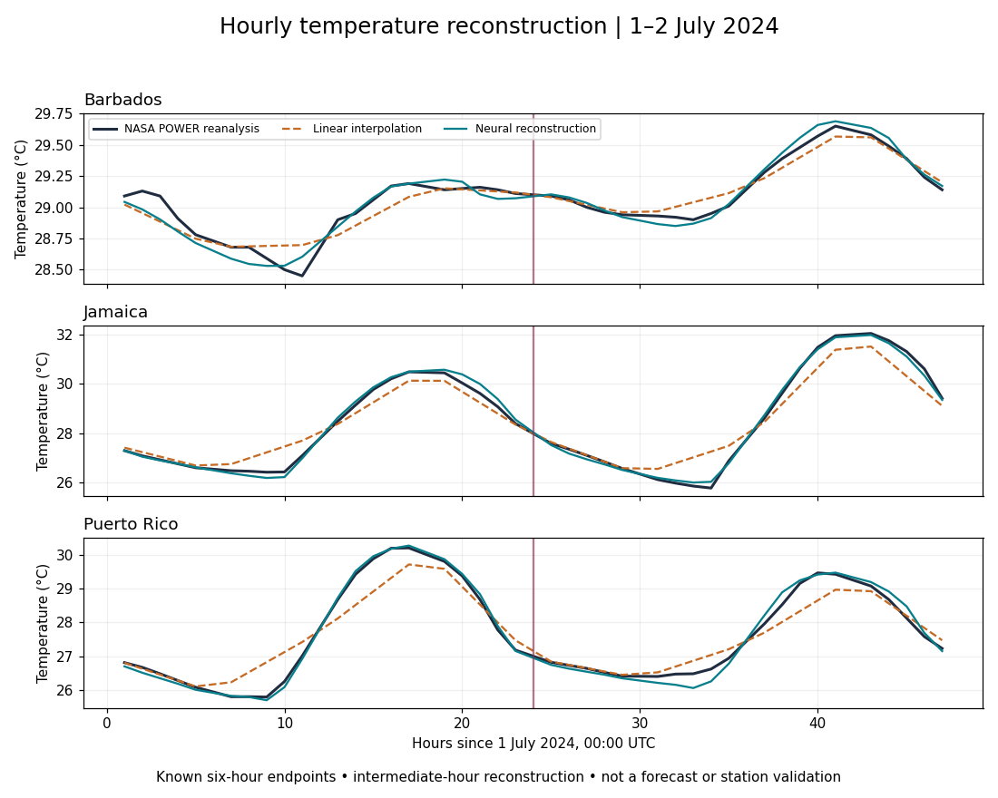
Both six-hour endpoints are supplied. Thus the task reconstructs intermediate values in a completed sequence; it does not predict an unknown future endpoint. Future observed endpoints would be unavailable to a forecast issued at the start. All three sites appear in the original pooled experiment. Here, leave-one-island-out comparisons exclude the evaluation island entirely from training and validation. No inference of Caribbean-wide performance follows from three individual coordinates.
Methods: matched models and ablations
The original location-aware network has 305 parameters. This extension uses the same two hidden layers, with 16 and 8 units, but removes latitude and longitude from every variant, giving 273 parameters. Inputs contain endpoint temperatures, fractional hour and cyclic hour/day coordinates. Normalisation is fitted only on training data for each split. Pooled results therefore address a different input specification from the original experiment.
The free residual model adds an unconstrained correction to interpolation. The endpoint model multiplies the correction by , forcing zero residual at . The supervised objective is where contains adjacent withheld hours within one six-hour interval. We compare . This is target-derived rate matching, not a heat equation or physics-informed neural network (PINN).
Each of four split settings uses three initialisations per candidate, 3,000 Adam steps, and checkpoints at 1,500 and 3,000 steps. Checkpoints and reported family representatives are selected by validation temperature RMSE. Positive-penalty winners are separately recorded per split and seed. Every candidate and seed is retained. The original evaluation years had already been inspected, so these additional comparisons are exploratory, not confirmatory.
Baselines include linear interpolation and a training-only month/hour correction pooled across available sites. A location-specific calendar cannot be estimated for an entirely unseen island. Shape-preserving piecewise-cubic interpolation (PCHIP) uses the surrounding known endpoint sequence, a richer information set than the two-endpoint networks; a two-endpoint smoothstep baseline is also retained.
Results
Table 1 reports temperature RMSE for the validation-selected representative of each family, not the lowest test error. Full MAE, bias, seed ranges, year and island breakdowns accompany the reproducible files.
| Evaluation | Linear | Calendar | Free | Endpoint | ||
|---|---|---|---|---|---|---|
| Pooled | 0.511 | 0.315 | 0.232 | 0.226 | 0.217 | 0.226 |
| Jamaica excluded | 0.565 | 0.344 | 0.395 | 0.421 | 0.416 | 0.427 |
| Barbados excluded | 0.125 | 0.505 | 0.439 | 0.497 | 0.499 | 0.499 |
| Puerto Rico excluded | 0.669 | 0.426 | 0.381 | 0.379 | 0.380 | 0.381 |
Barbados transfer is a clear failure relative to interpolation. Jamaica transfer is worse than the pooled calendar correction. Puerto Rico shows gains against both simple baselines. No penalty consistently improves accuracy across all locations. In the coordinate-free pooled setting, the selected rate-penalty model has RMSE 0.217 degrees Celsius, versus 0.226 for the endpoint model without that penalty; this comparison does not establish a causal physical advantage.
PCHIP gives pooled RMSE 0.401 degrees Celsius, compared with 0.518 for two-endpoint smoothstep. These additional baselines are weaker than the pooled neural variants here, but PCHIP’s different endpoint context must be acknowledged. Endpoint-model corrections vanish by construction, while free models need not reproduce supplied endpoints. This architectural property must not be presented as independent physical validation.
Discussion: physical interpretation and contribution
A two-metre air-temperature energy equation requires compatible treatment of advection, turbulent exchange, radiation, storage and unresolved sources. A surface energy budget is not automatically an atmospheric budget at two metres. Assigning arbitrary coefficients and reporting a small residual would demonstrate agreement with an assumed equation, not real physical consistency. Smoothness and endpoint agreement are insufficient grounds for the PINN label.
Weather downscaling with physical losses already exists, including Luo et al. [1]. Neural temporal interpolation of two-metre temperature is also established [2], [3]; hourly transformations based on daily summaries provide another baseline family [4]. CDAnet demonstrates physics-informed downscaling in numerical fluid convection [5], not independent validation of near-surface Caribbean weather. Adding a physical penalty or changing region alone is not a demonstrated new method.
The present contribution is a reproducible examination of constraint and transfer failure at three Caribbean points. A stronger journal study would need a sharper hypothesis, broader independent station coverage, a defensible physical closure with matched no-physics controls, and actual issued-forecast evaluation. Model complexity should be justified by demonstrable gains over simple methods, including adverse cases. No journal acceptance, comprehensive novelty or operational readiness is implied.
Limitations and future work
Preserve reanalysis reconstruction, actual forecast downscaling and station validation as separate experiments. Obtain regional fields and stations with compatible units, time stamps and licences. Define closure uncertainty explicitly; fit parameters only on training data. Compare identical architecture and forcing with physics disabled, and assess empirical error and physical residual separately. Hold out years, locations and heat events; evaluate peak timing, threshold duration and uncertainty calibration only where the model supplies the corresponding outputs.
The private evidence record retains all 48 fits, normalisation arrays, predictions, selection records, source hashes, gradient checks and adverse outcomes. The paired analytic gradient has a maximum finite-difference discrepancy of . Independent audit and exact-version review records are retained with the private evidence. This is an exploratory three-site study, not evidence of broad geographical transfer or spatial-resolution improvement.
Conclusion
The matched tests do not support a uniformly beneficial constraint or transferable neural reconstruction across the three locations. The excluded Barbados case favours interpolation, whereas Puerto Rico shows lower error with the neural variants. A physical interpretation requires additional forcing and closure evidence; a rate penalty alone does not supply it.
Data and code availability
Source responses, all model candidates, selection records and diagnostic outputs are retained privately. No public analysis archive is currently provided. The references identify the external methodological evidence, not a public download of this study’s trained models.
References
Luo et al. (2025). Physics-Guided Learning of Meteorological Dynamics for Weather Downscaling and Forecasting. ACM SIGKDD. https://doi.org/10.1145/3711896.3737081.
Wang et al. (2025). Neural Network Based on Dynamic Collaboration of Flows for Temporal Downscaling. Remote Sensing 17, 1434. https://doi.org/10.3390/rs17081434.
Serifi et al. (2021). Spatio-Temporal Downscaling of Climate Data Using Convolutional and Error-Predicting Neural Networks. Frontiers in Climate 3, 656479. https://doi.org/10.3389/fclim.2021.656479.
Hsiao (2024). Hourly temperature downscaling method based on clustering and linear transformation: Utilizing mean, maximum, and minimum temperatures. Energy and Buildings 325, 114975. Primary abstract inspected. https://doi.org/10.1016/j.enbuild.2024.114975.
Hammoud et al. (2022). CDAnet: A Physics-Informed Deep Neural Network for Downscaling Fluid Flows. JAMES 14, e2022MS003051. https://doi.org/10.1029/2022MS003051.