Keywords: atmospheric reconstruction; shared flux; model discrepancy; joint uncertainty; sparse observations; evaluation protocol.
Introduction
Atmospheric reconstruction estimates a past state using observations available within an event window. A physically balanced estimate is useful only if it also recovers quantities supported by independent evidence. The distinction matters in the Caribbean, where a regional reconstruction may rely heavily on a large-scale background between observations. The fifth-generation European Centre for Medium-Range Weather Forecasts reanalysis (ERA5) is an analysed product, not independent ground truth (Hersbach et al. 2020). This paper considers the hydrostatic, pressure-coordinate reconstruction class defined in Adrian Dunkley’s Chapter 3, dated 25 October 2026.
The thesis already distinguishes uncoupled fields, state matching, penalised flux matching and one shared signed interface transfer. It also proposes uncertainty from the background and model discrepancy. The present contribution is narrower than those ideas: specify the joint distribution of shared transfers, show which uncertainty claims follow from that specification, and define tests that can reject its practical value. Standard conservative and domain-decomposed learning methods precede this proposal (Jagtap, Kharazmi, and Karniadakis 2020; Moseley, Markham, and Nissen-Meyer 2023). Exact algebraic cancellation is consequently not claimed as new.
The research question is whether joint uncertainty in shared transfers improves the distribution of independently verified moisture tendencies and transport, compared with a matched face-local latent inference family, when observations are sparse and the background is biased. The primary estimand is the paired difference in an event-level probabilistic score under a fixed information set. Conservation error is a separate diagnostic, not a component of a score that could conceal poor reconstruction.
Evidence and scope
Physics-informed neural networks encode differential relations alongside observations (Raissi, Perdikaris, and Karniadakis 2019), but optimisation failures can prevent reliable solutions even for specified equations (Krishnapriyan et al. 2021). An incorrect equation presents a separate modelling risk. Hard-constrained downscaling shows how numerical constraints can be imposed architecturally (Harder et al. 2023); it does not establish that the imposed coarse total is unbiased. Weak-constraint assimilation explicitly allows model error (Trémolet 2006). ProbConserv already combines integral conservation constraints with probabilistic predictions and Bayesian updating (Hansen et al. 2023). Its results also show that improved likelihood or conservation need not improve every point-error metric. The proposed sub-analysis therefore does not originate probabilistic conservation: it isolates shared-transfer dependence within a particular atmospheric smoothing design.
Stochastic Separable Physics-Informed Neural Networks introduce low-rank representations over space, time and random inputs (Li and Onwunta 2026). Their reported benchmark performance motivates a candidate representation for uncertain transfers. The paper’s regular-domain bias and absence of a finite-rank end-to-end error guarantee remain material: a useful representation is not a calibrated atmospheric posterior. Hybrid atmospheric models such as the neural general circulation model NeuralGCM further demonstrate that physical structure and learned components can be combined, but their validation does not transfer to this proposed local smoother (Kochkov et al. 2024).
Optimistic Test-Time Adaptation adds a planning term to a world-model adaptation objective (Mete, Kalathil, and Kumar 2026). Its relevance here is limited to the mismatch between a training objective and the eventual evaluation target. A retrospective smoother has no licence to favour a desirable outcome. No optimistic planning loss is added to the likelihood or posterior below. The world-model paper’s task-dependent results are not evidence of atmospheric reconstruction skill.
Proper scoring rules assess predictive distributions rather than interval width alone (Gneiting and Raftery 2007). Joint evaluation also needs dependence-sensitive diagnostics because a plausible set of marginal distributions can conceal incorrect spatial dependence (Scheuerer and Hamill 2015). WeatherBench 2 provides a useful precedent for explicit evaluation conventions, although its forecasting benchmark is not the present smoothing task (Rasp et al. 2024).
State, observations and shared transfers
A bounded physical interpretation
Let the horizontal domain consist of non-overlapping columns. For column with area in , define water-vapour mass (1) where is specific humidity in , is gravitational acceleration in , and pressure is in pascals. Surface pressure, terrain masking and boundary uncertainty must be recorded. A precipitation-rate image is not this reservoir. Condensate storage, flux through the model top, surface-pressure effects and unresolved processes enter the documented discrepancy when they are not represented explicitly. Moisture-budget calculations are sensitive to discretisation and product consistency (Seager and Henderson 2013).
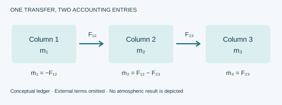
Orient each internal face once. Let be the node-edge incidence matrix, with at the receiving column and at the sending column. Let contain signed, face-integrated transfers in . The resolved accounting relation is (2) Here contains external boundary exchange, the specified column-integrated sources and sinks, and bounded model discrepancy; all have units . The orientation convention fixes every sign. A free discrepancy fitted independently at every point could absorb all error, so its form and prior must be fixed on development information and tested against adverse controls.
The information set remains retrospective
For latent atmospheric fields and observations , use , where represents footprint, time accumulation, vertical sensitivity and masking. Partition the observations into assimilated data and verification data . The target is ; may include later observations within the window, but never . This differs from a forecast distribution conditioned only on information available before an issue time. Products sharing gauges or retrieval inputs must not be treated as independent validation sources.
The atmospheric field determines compatible moisture masses and transfers. Independent networks for and cannot be called physically consistent merely because a penalty is small. A shared face functional must be documented, including quadrature, geometry and how both neighbouring fields enter it. Numerical conservation is checked after the actual time discretisation, not inferred from a continuous equation alone.
Analytical diagnostics
Conservation does not imply calibrated uncertainty
Proposition 1 (Samplewise ledger). If every internal face has one transfer used with opposite signs in its two columns, then internal transfers make no contribution to the domain-total tendency, for each ensemble member and not only in expectation.
Proof. Every column of contains one and one , hence . Premultiplying Equation 2 gives . The identity holds for any sampled . It says nothing about the accuracy of that sample or the external terms. ◻
For the implemented discrete update, use one time-integrated transfer in kilograms on both sides of every face: (3) where contains the integrated external terms in kilograms. Separate quadrature of the two sides would invalidate this discrete identity.
For an ensemble conditioned on the same assimilated observations and geometry, let . If the external terms are fixed, then (4) If external terms are random, their covariance and cross-covariance with must be included; independence is an assumption to test, not a default deduction. For the middle column in Figure 1, (5) Thus independent face samples can preserve exact conservation yet misrepresent local uncertainty. The sign and size of the error depend on the omitted covariance. Independent sampling is not necessarily overconfident: positive covariance makes the independence approximation too variable in this example, while negative covariance makes it too narrow.
Storage cannot identify every transport
Proposition 2 (Cycle ambiguity). Suppose observations constrain only the mass trajectory and the external terms in Equation 2. Any flux perturbation with leaves that trajectory unchanged. On a graph with a cycle, non-zero such perturbations exist.
Proof. Replace by . The change in mass tendency is . A circulating transfer around a closed cycle has one incoming and one outgoing contribution at each participating column, constructing a non-zero example. The likelihood of storage-only observations cannot distinguish these fluxes without additional assumptions or observations. ◻
This counterexample limits a transport-recovery claim even when a water-budget fit is exact. Independent wind or humidity-profile information may constrain the ambiguity; a prior can select a member of the equivalence class but does not convert that selection into observation-based identification. The argument concerns the ledger alone, not every dynamical constraint in the full atmospheric model.
A biased fixed background can produce false precision
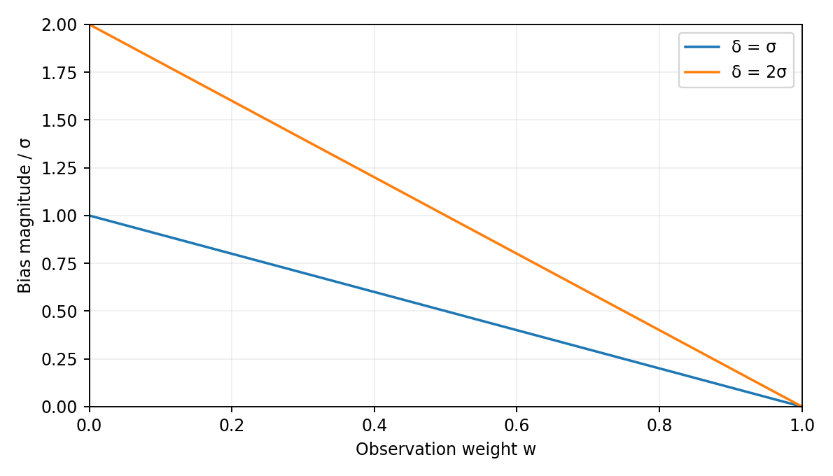
Consider a scalar illustration with fixed truth , observation , , and assumed Gaussian prior mean and variance . The posterior mean and its stated variance are (6) Under repeated observation noise with the biased background held fixed, (7) The last expression is frequentist mean-squared error under this stated experiment, not the posterior variance. As , reported variance tends to zero while bias tends to . This elementary counterexample motivates bias stress tests; it does not estimate atmospheric bias or establish that widening intervals will improve a proper score.
Proposed uncertainty specification
The candidate representation uses shared random coordinates rather than separately resampling each face. A low-rank expansion is (8) where is base noise independent of , and , under its fixed reference distribution. The coefficients are deterministic functions of in this conditional approximation. Orthonormal stochastic bases are established constructions (Xiu and Karniadakis 2002). Coefficients retain transfer units. These assumptions give at a fixed time. If assimilation instead updates the law of , the formula becomes for fixed coefficients, with the conditional basis mean added to . Reference orthogonality alone would then be insufficient. This positive-semidefinite covariance construction is standard, not a new theorem. Shared coordinates can represent dependence; they do not guarantee the correct dependence. Rank, basis order, reference distribution and parameter count are recorded and selected only on development data. The ensemble interpretation requires a specified conditional inference procedure, not merely random perturbations around a fitted mean.
Two tests must be kept separate. An algebra diagnostic holds all external terms fixed and independently permutes face draws, using each permuted draw on both sides of its face. It isolates the effect of covariance on local tendency spread while preserving the ledger. It is not a physically compatible posterior and cannot establish end-to-end reconstruction benefit.
The end-to-end comparison instead requires matched, valid conditional inference families: face-local latent innovations versus shared latent innovations, passed through the same state/flux-compatible reconstruction map. Both retain the same likelihood, boundary and discrepancy treatment, observation information, marginal calibration procedure and total tuning budget. The common physical map may itself induce dependence, so the first family must not be described as an independent-flux posterior. The exact map and restrictions are implementation gates; if matching them is infeasible, no practical-benefit claim follows from the permutation diagnostic.
One candidate sampler propagates uncertain boundary and prescribed-tendency draws through repeated constrained reconstructions. Compare its conditional moments and scores with a tractable reference problem before interpreting its members as conditional uncertainty. It is an approximation, not exact Bayesian sampling by definition. Rank and calibration are selected on separate development events and frozen before testing. A deterministic fit with a separately calibrated residual distribution remains an additional baseline.
Evaluation protocol
Development and withheld experiments
The first stage is an observing-system simulation experiment, meaning a controlled test where a separately generated reference state provides known truth (Hoffman and Atlas 2016). The reference generator must differ from the reconstruction backbone. Independent numerical and synthetic-observation errors are recorded. A simple finite-volume stochastic transport problem can check the ledger and covariance implementation before an atmospheric case, but cannot establish weather skill.
The second stage uses observed events with whole-event or contiguous-time holdouts. The thesis’s candidate domain and pressure levels remain proposals, not frozen choices. Event selection, observation inventory, background products, source licences, reference-generator identity and compute budget must be approved and documented before comparative evaluation. Background and observation transformations are fitted on training data only. Observation thinning uses predefined masks; repetitions of a mask or correlated grid cells do not create independent atmospheric events.
| Comparison | Controlled difference | Evidence required |
|---|---|---|
| Shared versus face-local latent family | Same compatible state/flux map; latent dependence differs | Joint scores, matched marginal calibration and explicit map verification |
| Joint versus calibrated deterministic baseline | Representation beyond post-hoc residual calibration | Proper-score improvement with sharpness and failure cases reported |
| Shared versus penalised flux | Samplewise accounting mechanism | Independent numerical ledger and withheld transport checks |
| Accurate versus perturbed background | Prespecified bias and boundary perturbations | Error, calibration and degradation curves across perturbation levels |
Outcomes and rejection criteria
For univariate quantities, use the continuous ranked probability score, which compares an estimated cumulative distribution with the realised observation. For multivariate vectors, report an energy score and a variogram score with weights and order fixed on development data (Gneiting and Raftery 2007; Scheuerer and Hamill 2015). Neither is sufficient alone to identify every error in dependence. Include interval coverage, interval width, marginal bias and selected covariance diagnostics. A distribution can obtain nominal coverage by becoming uninformatively wide; proper scores and sharpness prevent that observation from becoming the sole success criterion.
For the first controlled comparison, the proposed primary score is the energy score of a fixed vector of column moisture tendencies at prespecified verification times. Divide each component by its training-only scale, with a documented positive floor; average scores within an event before averaging events. The vector support and scaling remain identical for all models. A variogram score is a prespecified dependence-sensitive secondary outcome. With and denoting the shared-latent and face-local inference families, the primary contrast is (9) where is a prespecified event-aggregated proper score and lower is better. Fix normalisation, variable weights and spatial support before comparison. Report paired intervals using event-level resampling; within-event dependence may require a block method with block choice justified on development information. Künsch (Künsch 1989) is a source for follow-up on dependent resampling; only its metadata were verified for this draft, so no theorem or specific block rule is attributed to it. No sample size or detectable effect is asserted before a pilot and power assessment. Individual grid cells are not the sample size.
Coverage improvement alone does not establish practical value. A positive primary claim requires the upper endpoint of the paired interval for to fall below a pilot-defined negative benefit margin, frozen before held-out outcomes. Report the associated width, bias and secondary scores; wider intervals can legitimately correct underdispersion. Reject a claimed advantage that disappears under matched budgets or depends on shared validation inputs. Prespecified adverse trade-offs must remain visible rather than be averaged away. Report null and adverse outcomes. Ledger cancellation is checked to a tolerance derived from arithmetic and solver error; it is not credited as independently observed physical closure. When truth is unknown, withheld humidity and wind observations can test parts of the state but cannot establish an unobserved three-dimensional transport field.
Relationship to the thesis and existing work
Chapter 3 already contains the relevant uncertainty hypothesis. This paper supplies a proposed sub-analysis of it, not an additional claimed doctoral contribution. The shared-transfer covariance ablation belongs after the coupling variants; the cycle counterexample belongs in the identifiability discussion; the biased-background illustration belongs beside the uncertainty rationale. Source-specific insertion suggestions are supplied separately, leaving the current thesis unchanged.
The author’s earlier Closure-Limited, Evidence-Adaptive Residual Physics-Informed Neural Network (CLEAR-PINN) manuscript concerns precipitation-image nowcasting, bounded closure and synthetic component evidence. Its observed synthetic outcomes are not imported here. The present state is atmospheric water vapour, the task is smoothing, and the new testing emphasis is joint uncertainty in internal transfers. If later implementation reveals the same central estimand as another portfolio paper, these materials should be merged as a supplement rather than fragmented into another publication. Independent novelty review and supervisor agreement remain prerequisites to any external submission.
Limitations and conclusion
The analytical results are properties of a stated graph and scalar model. They do not prove non-negativity, stable atmospheric integration, identifiable fluxes or calibrated uncertainty. Hydrostatic reconstruction at a background-resolved scale cannot be described as convection-permitting simulation. Geometry, representation error, conditional-sampling quality and model discrepancy may dominate the uncertainty representation itself.
The protocol isolates a specific distinction: exact shared-transfer accounting and accurate joint uncertainty require different evidence. The ledger and cycle arguments explain why, while the proposed matched comparisons specify how practical benefit could be falsified. Until those comparisons are executed, no practical reconstruction gain is claimed.
Availability and declarations
This is a private, arXiv-style protocol draft, not an arXiv submission or a peer-reviewed article. No atmospheric dataset, numerical experiment or learned model was generated for this paper. Figure 2 evaluates an explicitly stated analytical expression; the other figures are conceptual. Editable LaTeX, source records, review records and the thesis proposal accompany the draft. Public sources retain their original licences.
This is a draft for author and supervisory review. No new funding, institutional approval, ethical approval or conflict declaration is asserted. The internal checks are not external peer review.