Keywords: rainfall planning; Jamaica; climatology; retrospective evaluation; moisture budget; physics-informed modelling.
Introduction
A planning framework should establish whether a fitted rainfall model improves on a simple reference before its outputs are used in agricultural or flood-impact calculations. It should also identify the temporal scale and observation process of its inputs. Monthly gridded estimates can support a historical planning comparison, but cannot establish minute-scale flood-warning skill.
This report asks whether a development-fitted blend of climatology and previous-year rainfall improves monthly agreement with a retained Jamaican rainfall product. Its contribution is a reproducible baseline comparison and a clearly bounded route towards physical modelling. The statistical replay, synthetic transport experiment and proposed atmospheric budget are separate evidence categories, rather than interchangeable demonstrations of forecast accuracy.
Data and methods
Historical rainfall and spatial support
The historical demonstration uses gridded rainfall estimates from Climate Hazards Center Infrared Precipitation with Stations version 3 (CHIRPS3), rather than simulated rainfall.
The retained subset contains 540 months, January 1981 to December 2025, on a 0.05-degree grid. A fixed Jamaica mask selects 374 cells. Its SHA-256 checksum matches the original acquisition manifest. The original October 2026 retrieval record lists provider files, timestamps and checksums; this extension rechecks the retained subset, rather than claiming a fresh download of all global files.
CHIRPS3 combines satellite information and station observations. Calling it “actual data” identifies a real provider dataset; it does not make each grid value a direct local measurement. Monthly support is appropriate for a planning demonstration, not minute-scale flash-flood warning. The existing field-data gap is independent rain gauges and, for flood applications, stream stage, discharge, inundation and local channel information.
Baseline specification and evaluation
A calendar-month climatology is fitted on 1981–2009. A second baseline repeats the same month’s rainfall from the previous year. Their convex blend is Here indexes target months, indexes grid cells, denotes calendar month, is training-period climatology, and is the previous year’s rainfall estimate for that cell and calendar month. All rainfall terms are in mm/month, and is dimensionless. Fixed nominal cell-area weights scale approximately with the cosine of cell-centre latitude and are normalised over the selected cells.
The coefficient is selected from a fixed grid with step 0.01 using area-weighted squared error on 2010–2016. The selected coefficient is 0.81 on climatology. The frozen model is then replayed on 108 months in 2017–2025. These years were already used in earlier research: they are a separate evaluation slice for this code, not a newly untouched scientific holdout.
The model uses no target-month rainfall as an input. The nominal issue time is the start of the target month, using climatology and a twelve-month lag. CHIRPS3 Final is normally produced in the following month’s third week. A twelve-month lag avoids assuming yesterday’s final product is already available, but the historical files are revised archives, not the actual product vintages available at each issue date. Accordingly, this is a retrospective replay, not a verified real-time forecast experiment.
Results
| Model | Root mean squared error | Mean absolute error |
| (mm/month) | (mm/month) | |
| Calendar-month climatology | 98.18 | 69.25 |
| Previous-year same month | 132.16 | 88.13 |
| Development-fitted blend | 98.73 | 69.52 |
Each month receives equal weight; spatial weights are fixed nominal cell areas. These errors measure agreement with CHIRPS3. The blend does not beat climatology on this historical evaluation slice. Retaining this result prevents a fitted model from being presented as an improvement merely because it is more complicated. A separate scalar accumulation reproduces the blend mean squared error. A deliberately leaked target-copy control obtains zero error, illustrating why target-input checks are necessary; it is not a legitimate competitor.
Only one rainfall product is used here. This extension therefore does not test the earlier cross-reference ranking claim on real data. A second aligned product and a documented dependence audit are needed for that question.
Physics-informed modelling framework
A physics-informed neural network is a neural function fitted with a differential-equation residual as well as data. The accompanying transport experiment has been executed: a 24-unit neural network fits a periodic one-dimensional field under . It compares the correct equation, no physics penalty and a deliberately wrong velocity. Later-time solution root mean squared errors are respectively 0.004672, 0.224283 and 0.559832 in dimensionless units. The wrong-velocity model has the smallest mass error despite its much larger solution error. This demonstrates why mass, equation residual and solution accuracy must be checked separately.
Those numerical results are synthetic transport reconstruction, not rainfall forecasts. The collocation domain includes the evaluated later times; future solution labels are withheld, but future-domain physics constraints are not. This distinction is retained when interpreting the animation. The experiment follows the general physics-informed residual formulation described by Raissi, Perdikaris and Karniadakis, while its deliberately broken equation addresses the need to test failure mechanisms rather than assuming that a physical loss guarantees a useful solution [1], [2].
A proposed rainfall-related extension would learn column water vapour and its horizontal transport under a moisture budget, Here is water mass per unit area (kg m), is vertically integrated horizontal water-vapour flux (kg m s), is evaporation, is precipitation and records unresolved budget closure (each in kg m s). This is a proposed budget constraint, not a new physical law or a trained rainfall model. Initial conditions, boundary fluxes, time-compatible atmospheric fields and closure assumptions must be specified before fitting. A freely adjustable could absorb every error, so it cannot be used to certify correctness. Identifiability and closure restrictions require explicit tests.
Monthly CHIRPS alone does not supply those atmospheric variables. The existing atmospheric research records provide a potential starting point, not validation of this proposed network. A prospective study would compare the network with the unchanged baseline and a conservative numerical model, separate reference dependence from physical residuals, and retain incorrect-equation controls. This work does not equate the synthetic PINN with the actual-rainfall statistical replay.
Discussion
The development-selected blend performs slightly worse than climatology on the evaluation period. This negative finding limits the case for adopting the extra lagged-rainfall component in this setting. It does not establish that climatology is optimal for other periods, regions or decisions. The comparison measures agreement with one gridded reference, while decision value would additionally depend on costs, thresholds and independent outcomes.
The transport experiment addresses a different question: whether a network can reproduce a prescribed synthetic evolution under correct and incorrect physical constraints. Its mass-error counterexample motivates separate diagnostic checks. It cannot supply the missing atmospheric observations or validate the monthly rainfall baseline.
Limitations
The evaluation period was used previously in the wider research programme, and historical product revisions prevent reconstruction of original issue-time information. Only one rainfall reference is assessed. No independent gauge, discharge, inundation or crop-response validation is supplied. Monthly temporal support and nominal cell-area weights limit local interpretation. The synthetic network has future-domain collocation constraints and must not be described as an operational forecasting test. The proposed moisture budget requires identified fluxes, boundary conditions and closure assumptions before it can be evaluated.
Future work
The proposed workflow is: acquire versioned rainfall and terrain inputs; record availability time and common spatial support; fit only on development periods; compare with simple baselines; preserve failures; then validate against independent field evidence before offering decisions.
Next work should obtain permitted local gauge records and their provenance, establish which gauges entered the reference product, and use fresh future evaluation periods. For operational testing, save forecasts at issue time and retain the input versions that were actually available. Compare multiple rainfall references on identical support. Test uncertainty, wet-season extremes, regional error and temporal stability rather than only average loss.
Agricultural planning further needs crop, soil, irrigation, cost and field-response information. Flood work needs sub-daily rainfall, drainage and river geometry, stage or discharge observations, and observed flood footprints. Terrain and satellite imagery alone cannot close those gaps. A physics-informed neural network can be evaluated inside the framework, but the separate synthetic transport experiment is not evidence of field-validated rainfall or flood skill.
Conclusion
The executed monthly comparison does not show an improvement over calendar-month climatology. Its value is to establish a transparent baseline and preserve the negative result before more complex models are introduced. Independent observations, availability-aware evaluation and separately checked physical diagnostics are necessary next steps for decision-oriented rainfall modelling.
Data and code availability
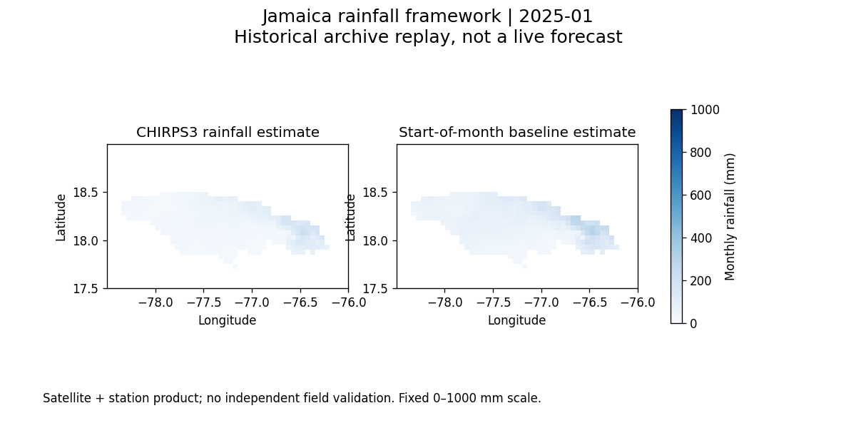
The private supporting research archive retains source provenance, acquisition checksums, the processed subset, baseline code, predictions, figures and computational reviews. The official dataset and documentation are available from the cited public providers; access to the private analysis archive is not implied. Earlier manuscripts and experiments are preserved. The animation is a historical replay and is not an additional measure of predictive skill.
Source documentation
Provider documentation checked 13 November 2026: https://www.chc.ucsb.edu/data/chirps3. Dataset citation: Climate Hazards Center, CHIRPS3 Data Repository (2025), https://doi.org/10.15780/G2JQ0P. The provider supplies reuse information on its documentation page; attribution is retained. Original source URLs and acquisition hashes accompany this report.
References
M. Raissi, P. Perdikaris and G. E. Karniadakis (2017). Physics Informed Deep Learning (Part I): Data-driven Solutions of Nonlinear Partial Differential Equations. https://arxiv.org/abs/1711.10561v1. Preprint; general residual formulation, not rainfall validation.
A. S. Krishnapriyan, A. Gholami, S. Zhe, R. M. Kirby and M. W. Mahoney (2021). Characterizing possible failure modes in physics-informed neural networks. NeurIPS. https://arxiv.org/abs/2109.01050v2. Supports the need to test optimisation and physical-loss failures; it does not validate the present numerical results.