Research question and contribution
Can a physically constrained neural solver reproduce a known transport solution, expose a deliberately wrong operator and preserve the distinction between actual forcing and observed outcomes? The first estimand is grid-averaged depth error on a dimensionless manufactured problem. The second is storage error against an analytic reservoir solution driven by acquired rainfall estimates. Neither is an estimate of emergency-warning performance.
This work presents an executable verification framework rather than a new hydraulic law or a demonstrated improvement in flood prediction. It reports two different settings: a controlled transport problem that permits exact error calculation, and a real-input calculation whose hydrological assumptions remain uncalibrated. Their connection is the audit procedure, not empirical evidence that one model transfers to a Jamaican river.
Related methods and evidence
Physics-informed neural networks represent differential-equation constraints in model fitting [1]. The present implementation belongs to the fixed-random-feature, output-layer least-squares family described by Dong and Li [2]; it does not train every hidden weight by gradient descent. This choice makes the first experiments small enough for independent calculation, while limiting what can be inferred about fully trained networks.
Constraint penalties can still fail. Krishnapriyan et al. examine failures on simple differential operators [3]. Wang et al. analyse unbalanced gradients [4] and mismatched convergence of loss components [5]. These findings motivate explicit broken controls and reporting of negative predictions, rather than equating a low residual with correct physical behaviour. The present experiments do not test the optimisation remedies proposed in those papers.
Hydraulic inundation models additionally require flow and momentum approximations, boundaries and friction. Bates et al. derive a reduced inertial shallow-water formulation [6]. A constant-velocity scalar transport equation or independent storage cell cannot substitute for that formulation. Here they isolate solver behaviour before any hydraulic interpretation.
CHIRPS combines satellite information with station blending [7], [11]. A Jamaican application analyses rainfall persistence and trends rather than validating flash-flood hydrographs [8]. The NOAA subset metadata identifies the exact daily product and units used here [12]. Copernicus documents a surface model that includes vegetation and infrastructure [13]. NASA’s IMERG documentation describes a separate half-hourly rainfall family with Early, Late and Final processing streams [14]; no IMERG array enters these experiments.
Earlier Jamaican research includes Mandal et al.’s assessment of warming thresholds and flooding in the Hope watershed [17]. Its catchment and climate-impact question differs from the numerical-verification question here; no result from that study is treated as validation of this model. The author’s earlier watershed feasibility memorandum separates daily runoff assessment from subhourly nowcasting and conditions catchment choice on station availability [18]. The present acquisitions progress that data-feasibility work, while leaving field performance as a separate empirical question.
Future field evaluation must respect dependence and spatial scale. Roberts et al. discuss blocked validation for structured data [9], and Roberts and Lean evaluate rainfall forecasts across spatial scales [10]. Their methods inform the proposed event/catchment split and scale-specific rainfall checks; they do not provide validation observations for this study. WRA’s service description and hydrologic guide establish a route to independent streamflow records [15], [16]. Actual station records must still be matched and assessed before evaluating a river model.
Manufactured problem
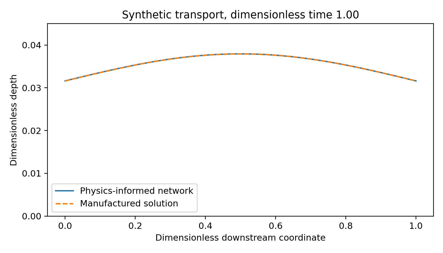
Let denote dimensionless distance and time, and let denote dimensionless depth. Set transport speed and solve The manufactured solution and its forcing are The forcing is positive on this domain. It is constructed from the solution rather than measured rainfall. The model is a linear transport surrogate; it lacks momentum, wetting and drying, infiltration, drainage structures and a calibrated relation between terrain and velocity. A dimensional interpretation would require stated length, time and depth scales. None is fitted to Jamaica.
The network is . Hidden weights are fixed Gaussian draws; biases are uniform on . Only is fitted. The least-squares objective combines 900 uniformly sampled interior residuals, 81 initial points, 81 inflow points and . Each boundary row and interior row has equal weight; the larger interior set therefore contributes more total weight. Configuration hashes are checked during reproduction. These runs were not prospectively preregistered. Seeds are 17, 29 and 41. Evaluation uses an regular grid. There is no tuning on that grid.
Executed comparisons
The wrong-velocity control fits the same forcing with ; the boundary-only control removes interior residuals. Their information differs deliberately. They diagnose residual dependence rather than provide a fair forecast contest against observed-data machine learning. All models share feature counts, initial and inflow data, seed and ridge strength.
| Model | Depth error range |
|---|---|
| Correct residual | – |
| Wrong velocity | – |
| Boundary only | – |
These ranges span three seeds, not confidence intervals. A central finite-difference derivative at 40 interior diagonal points () independently reproduces the analytic forcing to below maximum absolute error. The broken controls worsen depth error for every seed. Non-negativity of the target forcing is checked; the fitted depths nevertheless become slightly negative. Correct-residual minima are , and for seeds 17, 29 and 41. The soft residual therefore does not enforce depth positivity.
Numerical baseline and refinement
A first-order upwind discretisation of the same manufactured equation uses explicit forcing at the previous time and exact inflow values. The update is At spatial/time grid sizes , and , the Courant number is . Root mean square errors are , and respectively, with nonnegative grid values. Error decreases under joint refinement in this test. These are not equal-compute comparisons: the neural solution is fitted globally in space and time, whereas the explicit solver marches forward. No speed or general forecasting superiority is inferred.
Satellite rainfall and terrain inputs
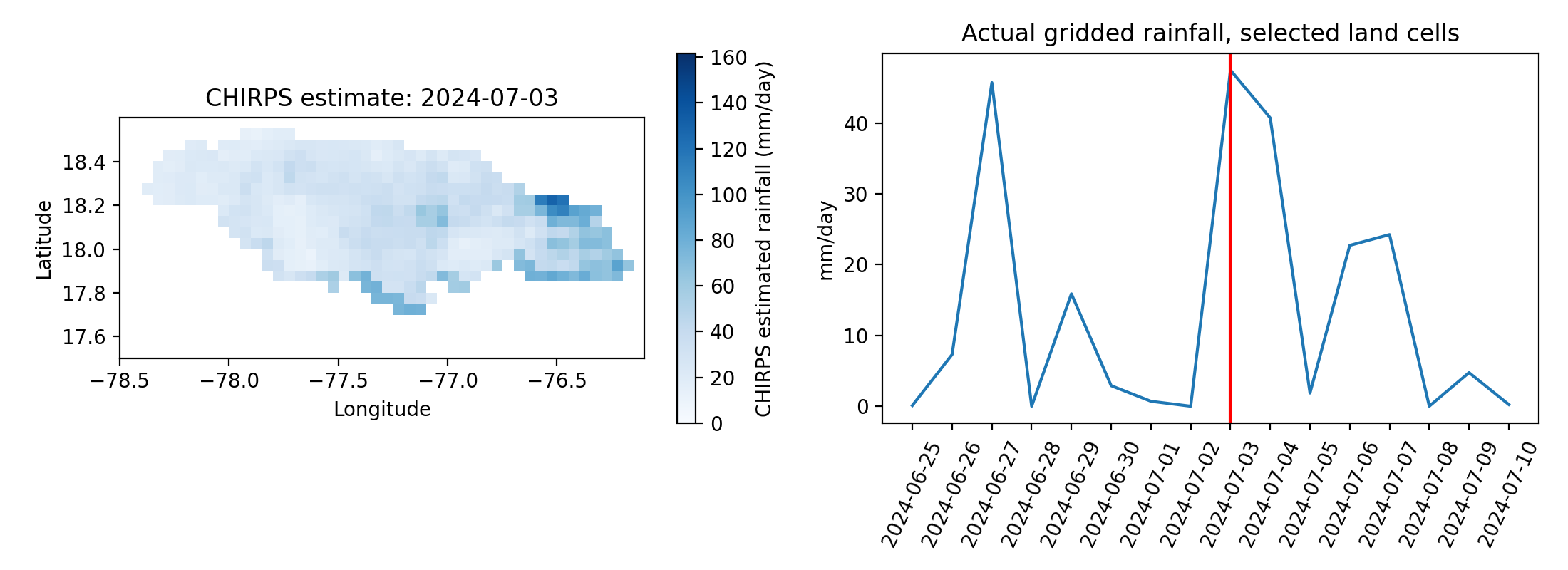
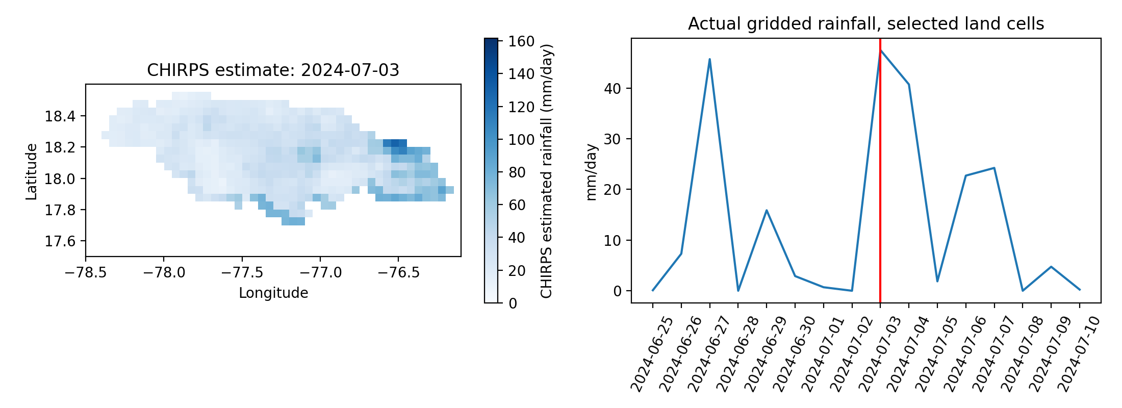
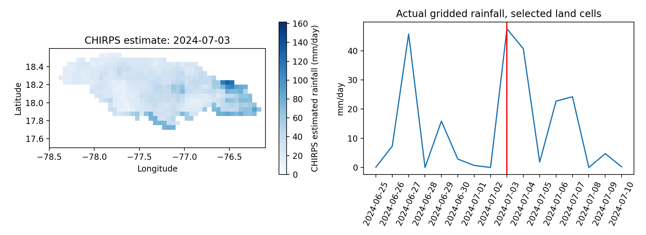
Sixteen consecutive daily rainfall fields, dated 25 June to 10 July 2024, were acquired from the NOAA ERDDAP mirror of the Climate Hazards Group InfraRed Precipitation with Station data (CHIRPS) product [7], [12], [11]. These are satellite-plus-gauge estimates, not direct rain-gauge truth. The retrieved box covers Jamaica and contains 7,040 finite land-cell/day estimates. Missing ocean cells remain missing. A second Copernicus elevation tile [13] extends the terrain coverage north of the original southeast tile.
The code intersects rainfall and terrain coverage, retaining 134 grid cells for a daily storage calculation. The rainfall animation and scenario figure report distinct quantities. The terrain enters the spatial selection and the elevation comparison plot; it does not determine calibrated routing or hydraulic parameters. The original physics-informed neural-network benchmark remains a manufactured-solution implementation test. A separate neural surrogate solves the assumed storage equation using the actual rainfall series as forcing; neither model has field-validated flash-flood performance.
Actual-forcing storage experiment
For grid cell , let be stored water volume in cubic metres, the estimated daily rain rate in millimetres per day, and the approximate spherical cell area in square metres. The assumed effective inflow is For each day of constant forcing, the exact update is Initial storage is zero. The runoff fraction and residence time are chosen assumptions, not fitted estimates. Cells are independent reservoirs; the domain is not a delineated catchment. Coast-intersecting cells use their full spherical area rather than a fractional land mask, which adds area uncertainty. There is no channel routing, momentum equation, inundation or exposure calculation.
The area-weighted peak rainfall estimate in the retained domain is mm/day. The largest accumulated water-budget discrepancy is cubic metres, a numerical balance check. It is not evidence of correct hydrology. Simulated aggregate outflow peaks at million cubic metres/day under the stated assumptions. This is not discharge measured at a river gauge, an estimate of floodwater depth, or a validated risk measure.
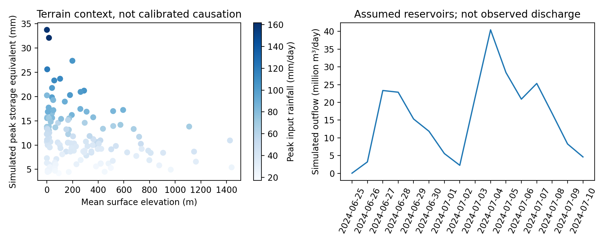
Physics-informed neural surrogate
A second executable fits a physics-informed, fixed-feature neural surrogate to the area-weighted actual rainfall series. It uses 32 random hidden features, seed 23 and 48 interior collocation points per day. Each day’s ordinary differential equation is solved on its own interval, passing the predicted ending storage to the next day. Only output weights are fitted; no observed discharge or storage targets are supplied.
Verification against the analytic reservoir solution at 25 points per day gives a storage root mean square error of mm and maximum error mm. These very small errors concern a simple, exactly specified linear equation. They do not measure rainfall accuracy or real flood skill. The physical assumptions are shared by both routes, so agreement cannot validate runoff fraction, residence time or the independent-cell representation. Executable code is retained in code/real_forcing_pinn.py; fixed weights and predictions are stored in real_forcing_pinn.npz.
Cross-method verification
The BootLoop procedure used here consists of recording inputs and settings, executing a model, independently recounting selected outputs, deliberately breaking an assumption and preserving the resulting failure. It is a project audit procedure, not a new learning algorithm. The transport forcing was checked using centred finite differences at 40 interior diagonal points. A separate evaluator reconstructed saved neural predictions and calculated finite-difference residuals over the seed-17 grid. Fresh executions reproduced the reported per-seed metrics. The actual-input reservoir was recounted using its closed-form balance, and the storage surrogate was reconstructed from its saved hidden and output weights.
The numerical agreement has a narrow meaning. The reservoir solver and neural surrogate share the same rainfall, runoff fraction and residence time. Their agreement cannot test those assumptions. Likewise, the transport model uses its complete interior forcing during solution fitting; this is not a causal held-out forecast experiment. Reproduction records distinguish the initial configuration written before fitting from later hash-checked reruns, without claiming retrospective preregistration.
Field evaluation and future work
A defensible next experiment would select one gauged catchment and an event list before inspecting errors. Daily rainfall and daily streamflow can support a daily water-budget assessment. They cannot establish the within-day peak, arrival time or depth of a flash flood. That requires subdaily forcing, stage or discharge with rating-curve information, reliable timestamps, terrain-conditioned drainage and independently checked inundation.
The WRA guide describes daily streamflow downloads and flags that require explicit handling [16]. For streamflow, represents no-flow/dry conditions and denotes Hermitage Dam at capacity; older zero values may be ambiguous. These semantics differ from missing rainfall pixels and must not be treated as a universal missing-value rule. No WRA hydrograph was used here.
The catchment experiment should compare a hydraulic or rainfall-runoff numerical model, simple statistical baselines, matched unconstrained learning and a physics-informed model with equal issue-time information. Split by event and catchment where possible. Report peak magnitude and timing, depth and inundation errors, positivity, water-budget residual, lead time and computational cost, with event-block uncertainty. Calibration and evaluation must use independent periods. Any reference that shares gauges or rainfall inputs with the fitted product needs a dependence audit.
Terrain conditioning must inspect riverbeds, culverts, roads, buildings and vegetation. The two acquired surface-model tiles are not surveyed channel geometry. The present coarse neighbourhood aggregation clips at tile edges and uses full area for coastal rainfall cells. Neither boundary treatment has been calibrated to a catchment. Flood risk also requires exposure and vulnerability; this study produces neither monetary loss nor population-risk estimates.
Discussion and conclusion
The manufactured experiment shows that the chosen neural representation can solve a smooth transport problem and that the stated negative controls expose wrong or absent interior physics. The actual-input experiment demonstrates traceable acquisition, unit conversion, calculation and numerical verification using Jamaican rainfall estimates. Neither result establishes an operational flood model.
The main practical distinction is between a solver that agrees with its governing assumptions and a model that agrees with independently observed events. The former has been tested here. The latter defines the next empirical study. Animations expose changes in the retained fields but add no independent evidence of predictive skill.
Data and code availability
The reproducibility package includes acquisition URLs and hashes, input subsets, configurations, executable NumPy code, saved weights and predictions, metrics, figures and animations. CHIRPS source metadata and product version accompany the rainfall subset. No personal records are used. The modelling scope is numerical verification with retrospective gridded inputs, not an issued flood forecast.
Data attribution.
Terrain-derived analysis is produced using Copernicus WorldDEM-30 Copyright DLR e.V. 2010–2014 and Copyright Airbus Defence and Space GmbH 2014–2018 provided under COPERNICUS by the European Union and ESA; all rights reserved. Neither the licensor nor entities responsible for Copernicus delivery are liable for the derived analysis. CHIRPS data are supplied by the Climate Hazards Center and retained with their public-domain source notice.
References
M. Raissi, P. Perdikaris and G. E. Karniadakis (2017). Physics Informed Deep Learning (Part I): Data-driven Solutions of Nonlinear Partial Differential Equations. https://arxiv.org/abs/1711.10561v1.
S. Dong and Z. Li (2021). Local extreme learning machines and domain decomposition for solving linear and nonlinear partial differential equations. Computer Methods in Applied Mechanics and Engineering. https://doi.org/10.1016/j.cma.2021.114129.
A. Krishnapriyan et al. (2021). Characterizing possible failure modes in physics-informed neural networks. NeurIPS 34. https://arxiv.org/abs/2109.01050.
S. Wang, Y. Teng and P. Perdikaris (2020). Understanding and mitigating gradient pathologies in physics-informed neural networks. https://arxiv.org/abs/2001.04536v1.
S. Wang, X. Yu and P. Perdikaris (2020). When and why PINNs fail to train: A neural tangent kernel perspective. https://arxiv.org/abs/2007.14527v1.
P. D. Bates, M. S. Horritt and T. J. Fewtrell (2010). A simple inertial formulation of the shallow water equations for efficient two-dimensional flood inundation modelling. Journal of Hydrology 387, 33–45. https://doi.org/10.1016/j.jhydrol.2010.03.027.
C. Funk et al. (2015). The climate hazards infrared precipitation with stations—a new environmental record for monitoring extremes. Scientific Data 2, 150066. https://doi.org/10.1038/sdata.2015.66.
C. Avalon Cullen and R. Al Suhili (2023). Assessing Rainfall Variability in Jamaica Using CHIRPS: Techniques and Measures for Persistence, Long and Short-Term Trends. Geographies 3, 375–397. https://doi.org/10.3390/geographies3020020.
D. R. Roberts et al. (2017). Cross-validation strategies for data with temporal, spatial, hierarchical, or phylogenetic structure. Ecography 40, 913–929. https://doi.org/10.1111/ecog.02881.
N. M. Roberts and H. W. Lean (2008). Scale-Selective Verification of Rainfall Accumulations from High-Resolution Forecasts of Convective Events. Monthly Weather Review 136, 78–97. https://doi.org/10.1175/2007MWR2123.1.
Climate Hazards Center. CHIRPS2 product documentation and data policy. https://chc.ucsb.edu/data/chirps/.
NOAA ERDDAP. CHIRPS Version 2.0 daily precipitation: retained subset metadata. https://upwell.pfeg.noaa.gov/erddap/info/chirps20GlobalDailyP05/index.csv.
Copernicus Data Space Ecosystem. Copernicus DEM: Global and European Digital Elevation Model. https://dataspace.copernicus.eu/explore-data/data-collections/copernicus-contributing-missions/collections-description/COP-DEM.
NASA Global Precipitation Measurement Mission. Integrated Multi-satellitE Retrievals for GPM. https://gpm.nasa.gov/data/imerg.
Water Resources Authority, Jamaica. Services: resource monitoring and flood monitoring. https://www.wra.gov.jm/services/.
Water Resources Authority, Jamaica. Jamaica’s Water Information System: Hydrologic Database User Guide. https://webmap.wra.gov.jm/webmap/app/db/WRA%20Hydrologic%20Database%20User%20Guide.pdf.
A. Mandal, T. Stephenson, J. Campbell, M. Taylor, S. Watson, L. Clarke, D. Smith, J. Darsan and M. Wilson (2022). An assessment of the impact of 1.5 versus 2 and 2.5C global temperature increase on flooding in Jamaica: a case study from the Hope watershed. Philosophical Transactions A 380, 20210141. https://doi.org/10.1098/rsta.2021.0141.
A. Dunkley (2026). Jamaica Watershed and Earth Engine Data Feasibility Assessment. A companion to E001—Jamaica Extreme Rainfall Nowcasting. Unpublished data-feasibility memorandum, Climate Studies Group Mona, 22 October.