Keywords: Jamaica; satellite imagery; diffusion models; generative ensembles; rainfall; temperature; CHIRPS; MODIS; CRPS.
Evidence class: satellite imagery and products. NASA GIBS browse imagery (MODIS and IMERG layers), CHIRPS v2 daily rainfall, NASA POWER 2 m temperature and MODIS land-surface temperature, 2008 to 2025. No gauges and no synthetic data are used.
Introduction
A satellite image of Jamaica taken this morning contains information about tomorrow’s rain. Cloud tops, column moisture, the surface temperature of the land and the rain already falling are all visible from orbit, and a forecaster reads them by eye. The question this paper asks is whether a computer-vision model can read them too. Given the day’s satellite imagery and nothing else about the atmosphere, how well can a generative image model predict the next day’s rainfall and temperature fields across the island, does the imagery add anything beyond what yesterday’s fields and the season already say, and does the result survive comparison with probability forecasts that use no model at all?
Three choices define the study. The model is a conditional denoising diffusion model (Ho, Jain, and Abbeel 2020), the class of generative model that now underlies kilometre-scale downscaling (Mardani et al. 2025), radar nowcasting (Leinonen et al. 2023; Gao et al. 2023) and global probabilistic forecasting (Price et al. 2025). It produces an ensemble of plausible next-day fields instead of one blurred estimate, so its uncertainty can be scored. The inputs are images in the ordinary sense, true-colour composites from two MODIS overpasses and four derived satellite layers, fetched as pictures from NASA’s imagery service and decoded back to physical values where a colour map allows it. And the targets are the gridded products a Jamaican climate study would use anyway, CHIRPS daily rainfall at 0.05 ° and a 2 m air-temperature analysis, plus the satellite’s own land-surface temperature.
As in the earlier studies in this series, the test is strict. The model is compared with persistence, a day-of-year climatology, a per-pixel ridge regression on the same inputs and a deterministic UNet of the same architecture trained with a squared-error loss, all on the same 730 held-out days of 2024 and 2025, which include Hurricane Beryl, Tropical Storm Rafael and Hurricane Melissa. Its probabilistic scores are then set against four reference distributions built from the observations alone (a day-of-year climatological distribution, a Markov-chain climatology, a lagged ensemble and dressed persistence), because an ensemble scored only against point forecasts is rewarded for being a distribution, whatever it knows. The first evaluation of this experiment made only the first comparison; the second is new in this version and changes the conclusion. The diffusion model is also queried with its imagery channels switched off, so the contribution of the pictures can be separated from the contribution of the previous day’s fields. Every number reported is recomputed from the saved prediction files, and the negative parts of the result are kept.
Related work
Generative diffusion models entered weather and climate work through downscaling and nowcasting. Addison et al. (2022) and Harris et al. (2022) showed that generative models can produce realistic high-resolution rainfall conditioned on coarse fields, and the residual-correction formulation of CorrDiff (Mardani et al. 2025) made kilometre-scale downscaling of a regional analysis routine. For nowcasting from radar, LDCast (Leinonen et al. 2023) and PreDiff (Gao et al. 2023) replaced the adversarial training of DGMR (Ravuri et al. 2021) with latent diffusion and reported better calibrated ensembles; DuoCast (Wen et al. 2024) splits the problem by spatial frequency. GenCast (Price et al. 2025) extended the approach to global medium-range forecasting. Closest to the present study, Chase et al. (2025) nowcast geostationary infrared imagery itself with score-based diffusion, and DiffObs (Stock et al. 2024) rolled a diffusion model forward on daily IMERG precipitation globally. Watt and Mansfield (2024) applied diffusion downscaling to temperature and winds over the United States.
None of these targets a small tropical island, conditions on multi-sensor daytime imagery decoded from pictures, or predicts rainfall and temperature together at daily range. The Caribbean literature on satellite rainfall concerns product accuracy, with CHIRPS over Jamaica assessed against gauges (Cullen and Al Suhili 2023) and IMERG’s regional characteristics documented in its product papers (NASA Global Precipitation Measurement Mission 2026). Prediction from the imagery itself has not been attempted for the region. The earlier papers in this series established the local baselines a learned model has to beat for daily rainfall under stale inputs and scarce labels, and the conditions under which a small neural model is worth preferring to a linear one. The present paper applies that discipline to a generative image model.
Data
Window and grids
The window is 17.6 ° N–18.8 ° N, 78.5 ° W–76.1 ° W, which holds Jamaica with a margin of sea on every side. Imagery is fetched on a 96 by 48 pixel grid (0.025 °, about 2.7 km) and targets live on the 48 by 24 CHIRPS grid (0.05 °). The 440 CHIRPS cells with finite values define the land mask; rainfall is scored on those cells only. The period is 1 January 2008 to 31 December 2025.
Satellite imagery
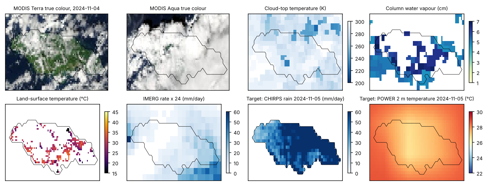
Six daily layers were fetched from NASA’s Global Imagery Browse Services (GIBS) through its WMS endpoint (NASA Earthdata 2026), one image per layer per day. They are the MODIS Terra and MODIS Aqua corrected-reflectance true-colour composites (morning and early-afternoon overpasses), the MODIS Terra daytime cloud-top temperature and column water vapour products (Platnick et al. 2017), the MODIS Terra daytime land-surface temperature (Wan 2014), and the IMERG daily precipitation-rate layer (NASA Global Precipitation Measurement Mission 2026). True-colour images are used as RGB. The four palette layers were decoded to physical values with the GIBS colour maps (nearest palette entry, bin midpoint), which gives cloud-top temperature in kelvin at 1 K to 6 K resolution, water vapour in centimetres, land-surface temperature in kelvin and rain rate in mm/h with 222 logarithmically spaced bins. Pixels rendered transparent (clear sky for cloud products, cloud for the surface product, below 0.1 mm/h for rain) are carried as a separate mask channel. Across the period the cloud-top layer is defined on 62 % of pixels, water vapour on 47 % and land-surface temperature on 11 % (29 % of land pixels). Thirty-one days in November and December 2022 have no true-colour imagery in the service and are dropped, leaving 6,543 imaged days.
Targets
Three next-day fields are predicted. Rainfall is CHIRPS v2.0 daily (Funk et al. 2015), read for the window from the IRI Data Library mirror. Air temperature is the NASA POWER daily 2 m temperature (NASA POWER 2026), a MERRA-2-based product on a 0.5 ° by 0.625 ° grid, interpolated bilinearly to the target grid. It is a coarse, smooth field and is treated as such in the discussion. Land-surface temperature is the MODIS layer above averaged 2 by 2 onto the target grid, available on 45 % of land cells on an average day and missing under cloud. The model is trained and scored on observed cells only.
Each sample pairs day with day : the conditioning holds the six imagery layers of day , the three target fields of day (with the land mask and the land-surface observation mask) and the day of year. The output is the three fields of day . There are 6,541 pairs: 5,114 for training (2008 to 2021), 697 for validation and model selection (2022 to 2023) and 730 for the test (2024 to 2025). Rainfall is modelled as and the three fields are standardised with training-period statistics (rain in log units; air temperature °C; land-surface temperature °C). The test years have a mean land rainfall of 4.32 mm/day; 14.7 % of land cell-days exceed 10 mm and 3.9 % exceed 25 mm.
Methods
Conditional diffusion model
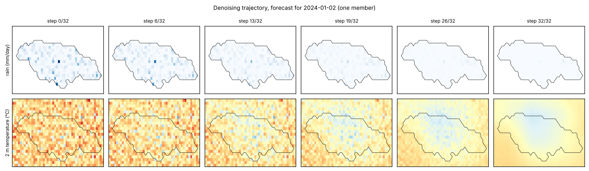
The model follows the denoising diffusion probabilistic framework (Ho, Jain, and Abbeel 2020) with the cosine noise schedule of Nichol and Dhariwal (2021) over steps. The network predicts the velocity (Salimans and Ho 2022) rather than the noise . A first run with -prediction and the same budget denoised poorly at high noise levels (its implied at had an error of 2.4 standard units) and its DDIM trajectories drifted to samples with 2.6 times the climatological spread, so the run was discarded and the parameterisation changed before any test score was computed. The network is a UNet (Ronneberger, Fischer, and Brox 2015) on the 24 by 48 target grid with widths 40, 80 and 160 at three resolutions, one residual block per level on each side and two at the 6 by 12 bottleneck with a self-attention block, and a sinusoidal time embedding; it has 1,739,787 parameters. The 13 imagery channels at 48 by 96 pixels enter through a strided convolutional encoder to 24 channels at target resolution and are concatenated with the noisy field and the seven low-resolution conditioning channels, the conditioning route used by CorrDiff and GenCast. The loss is the squared error on averaged over observed target cells (land for rainfall, all cells for air temperature, observed cells for land-surface temperature); unobserved cells contribute nothing.
Training uses AdamW (learning rate , weight decay ), batches of 32, gradient clipping at 1, a cosine learning-rate decay over 40 epochs, and imagery dropout: for 20 % of training samples the 13 imagery channels are set to zero, so the trained network can be queried with or without pictures. The checkpoint with the lowest validation loss (the same objective on the 2022 to 2023 pairs with fixed noise draws) is kept. Sampling uses the deterministic DDIM sampler (Song, Meng, and Ermon 2021) with 32 steps, the denoised estimate clipped to standard units at each step. An ensemble of 12 members is drawn per day from independent Gaussian initialisations, and fields are mapped back to physical units (rainfall capped at 500 mm/day). Sampler settings were fixed from a 24-day validation check and not tuned on the test years. Everything ran on two CPU cores; training took about 50 minutes and the test ensembles about half an hour.
Reference forecasts
Five references are scored on the same days and cells. Persistence repeats the day- field (for land-surface temperature, the day-of-year climatology fills cells that were cloudy on day ). Climatology is the mean of the training-period target within 15 days of the day of year, per cell. Ridge regression fits one linear model per cell and target on 20 features (the 13 imagery channels averaged to target resolution and the seven low-resolution channels), with the penalty chosen on the validation years from (1.0 was chosen). The deterministic UNet is the same network as the diffusion model with and a zero noisy input, trained for 20 epochs on the masked squared error of the standardised target. It is the direct test of whether generating rather than regressing changes the result. The imagery ablation queries the trained diffusion model with its 13 imagery channels zeroed, which leaves yesterday’s fields and the season as the only information.
Probabilistic references
The CRPS of a point forecast is its absolute error, and its Brier score is that of a 0/1 exceedance. Both penalise the absence of a distribution, so a comparison of an ensemble with point forecasts cannot show that the ensemble carries information. Four reference distributions are therefore built from the observations alone, with no learned parameters (Wilks 2019). The climatological distribution is, for each cell, the empirical distribution of the training-period targets whose image day falls within 15 days of the test image’s day of year, about 430 values. The Markov-chain climatology restricts that sample to training days on which the cell’s previous-day rainfall was in the same state as on the test day (below 1 mm, 1 to 10 mm, or 10 mm and above), and falls back to the unconditional sample where fewer than ten analogues exist. Conditioning occurrence on the previous day’s state is the classical first-order model of daily rainfall (Gabriel and Neumann 1962). The lagged ensemble takes the observed fields of the twelve most recent days as its twelve members (Hoffman and Kalnay 1983). For 2 m temperature, dressed persistence adds to the previous day’s field the empirical distribution of training-period one-day changes in the same 31-day window.
All four use information available at issue time and are scored with the same fair CRPS and Brier definitions on the same 730 days and cells. They were computed after the first evaluation, from targets fetched again from the same public sources. The rebuilt targets reproduce the archived deterministic scores: the climatological-mean rainfall RMSE is 9.798 against an archived 9.798 mm/day, persistence rainfall RMSE 12.402 against 12.402, and persistence temperature MAE 0.2553 against 0.2553 °C. That agreement is the check that both evaluations score the same data. The per-day ensemble scores of the archived run were not available to this analysis, so the comparison uses the model’s archived aggregate scores and carries no paired interval.
Scores and uncertainty
Fields are scored in physical units on observed cells of the 730 test days, with root-mean-square error (RMSE) and mean absolute error (MAE) of the ensemble mean, the fair continuous ranked probability score (CRPS) of the ensemble (Gneiting and Raftery 2007; Ferro 2014), which reduces to MAE for a deterministic forecast, and the mean ensemble standard deviation as the spread (Fortin et al. 2014). Rainfall also carries the fractions skill score at a 3 by 3 cell window for 10 mm and 25 mm thresholds (Roberts and Lean 2008), computed from ensemble exceedance probabilities, the Brier score for the same thresholds, and the RMSE and bias of the daily island-mean rainfall. Paired differences between the diffusion ensemble and each reference are given 95 % intervals from a 30-day block bootstrap over test days with 1,000 draws. Twelve members and 730 days bound how finely the ensemble can be assessed; the intervals are descriptive.
Results
Scores on the 2024 to 2025 test years
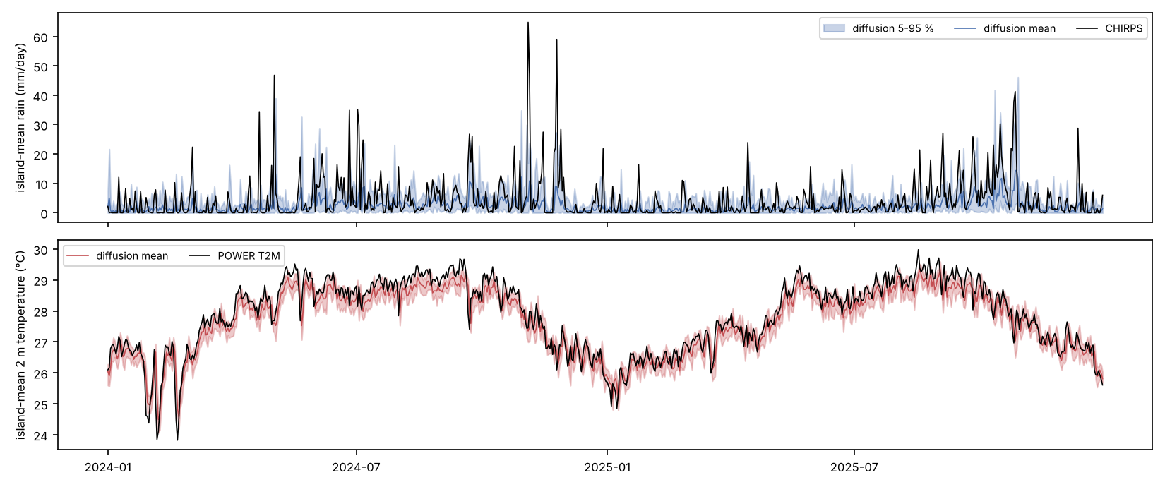
Table 1 gives the scores and Table 3 the paired differences. Among the trained models and the deterministic references, the diffusion ensemble has the lowest CRPS for all three targets, and every one of those differences has a bootstrap interval that excludes zero. For rainfall its CRPS of 3.287 mm/day is 23.3 % below the best deterministic reference (the UNet’s MAE of 4.288) and 37.6 % below persistence. For 2 m temperature it is 0.217 °C against 0.255 °C for persistence (15.1 % lower), and for land-surface temperature 2.17 °C against 2.67 °C for climatology (18.5 % lower).
Point accuracy is a different matter. On rainfall RMSE the diffusion mean (9.798) ties the day-of-year climatology (9.798; paired difference with interval ) and beats ridge and the UNet by about 0.51 mm/day, while on MAE the UNet (4.288) and ridge (4.332) are better than the ensemble mean (4.509), as a regression that shrinks towards dry days should be. On 2 m temperature the ensemble mean is worse than persistence by 0.040 °C with interval , and worse than ridge and the UNet by similar margins. On land-surface temperature it is worse than climatology by 0.26 °C with interval and indistinguishable from ridge and the UNet. Whatever the generative model contributes lies in the distribution it produces, since its point forecast is no better than the references. Section 5.2 tests that distribution against others.
| Rainfall (mm/day) | 2 m temperature (°C) | Land-surface temp. (°C) | ||||||||||
|---|---|---|---|---|---|---|---|---|---|---|---|---|
| 2-5(lr)6-9(lr)10-13 Method | RMSE | MAE | CRPS | spread | RMSE | MAE | CRPS | spread | RMSE | MAE | CRPS | spread |
| Persistence | 12.402 | 5.271 | 5.271 | – | 0.339 | 0.255 | 0.255 | – | 4.735 | 3.213 | 3.213 | – |
| Climatology | 9.798 | 5.377 | 5.377 | – | 0.883 | 0.776 | 0.776 | – | 4.010 | 2.665 | 2.665 | – |
| Per-pixel ridge | 10.311 | 4.332 | 4.332 | – | 0.345 | 0.268 | 0.268 | – | 4.249 | 2.851 | 2.851 | – |
| Deterministic UNet | 10.307 | 4.288 | 4.288 | – | 0.342 | 0.268 | 0.268 | – | 4.131 | 2.755 | 2.755 | – |
| Diffusion, imagery off | 9.970 | 4.535 | 3.337 | 3.878 | 0.380 | 0.303 | 0.216 | 0.238 | 4.317 | 3.102 | 2.196 | 3.652 |
| Diffusion ensemble | 9.798 | 4.509 | 3.287 | 3.945 | 0.379 | 0.304 | 0.217 | 0.237 | 4.269 | 3.053 | 2.171 | 3.583 |
| FSS, 3 by 3 window | Brier score | Island-mean rain (mm/day) | ||||
|---|---|---|---|---|---|---|
| 2-3(lr)4-5(lr)6-7 Method | 10 mm | 25 mm | 10 mm | 25 mm | RMSE | bias |
| Persistence | 0.468 | 0.280 | 0.1775 | 0.0604 | 7.82 | -0.01 |
| Climatology | 0.034 | 0.000 | 0.1520 | 0.0390 | 6.95 | -0.54 |
| Per-pixel ridge | 0.007 | 0.000 | 0.1464 | 0.0390 | 7.55 | -3.26 |
| Deterministic UNet | 0.007 | 0.000 | 0.1463 | 0.0390 | 7.55 | -3.33 |
| Diffusion, imagery off | 0.296 | 0.104 | 0.1226 | 0.0371 | 7.04 | -2.19 |
| Diffusion ensemble | 0.325 | 0.132 | 0.1204 | 0.0365 | 6.83 | -2.07 |
| Target | Reference | RMSE | 95 % interval | CRPS | 95 % interval |
|---|---|---|---|---|---|
| Rainfall | persistence | -2.604 | [-3.383, -1.957] | -1.984 | [-2.304, -1.676] |
| Rainfall | climatology | +0.000 | [-0.170, +0.160] | -2.090 | [-2.473, -1.764] |
| Rainfall | ridge | -0.513 | [-0.782, -0.259] | -1.045 | [-1.360, -0.774] |
| Rainfall | UNet | -0.509 | [-0.739, -0.291] | -1.001 | [-1.313, -0.747] |
| Rainfall | imagery off | -0.172 | [-0.342, -0.006] | -0.050 | [-0.114, +0.005] |
| 2 m temperature | persistence | +0.040 | [+0.020, +0.060] | -0.038 | [-0.056, -0.020] |
| 2 m temperature | climatology | -0.503 | [-0.581, -0.428] | -0.559 | [-0.639, -0.484] |
| 2 m temperature | ridge | +0.034 | [+0.020, +0.050] | -0.052 | [-0.064, -0.037] |
| 2 m temperature | UNet | +0.037 | [+0.028, +0.046] | -0.051 | [-0.059, -0.044] |
| 2 m temperature | imagery off | -0.001 | [-0.007, +0.004] | +0.000 | [-0.003, +0.004] |
| Land-surface temp. | persistence | -0.466 | [-0.669, -0.268] | -1.042 | [-1.215, -0.891] |
| Land-surface temp. | climatology | +0.259 | [+0.075, +0.456] | -0.494 | [-0.617, -0.366] |
| Land-surface temp. | ridge | +0.020 | [-0.160, +0.192] | -0.679 | [-0.823, -0.548] |
| Land-surface temp. | UNet | +0.138 | [-0.060, +0.344] | -0.584 | [-0.723, -0.431] |
| Land-surface temp. | imagery off | -0.047 | [-0.112, +0.019] | -0.024 | [-0.066, +0.016] |
Scores against probabilistic references
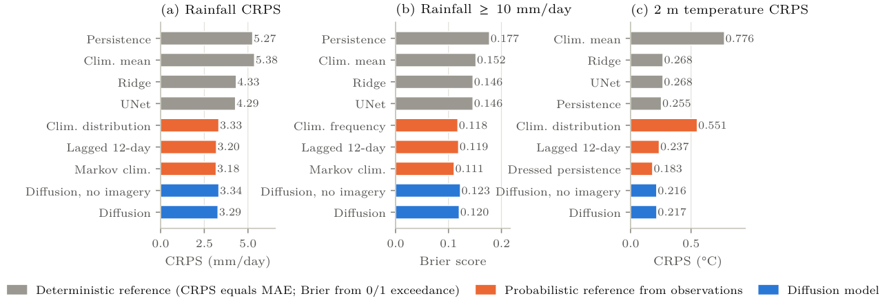
Table 4 and Figure 1 repeat the probabilistic comparison against the reference distributions of Section 4.3, and most of the advantage in Table 1 disappears. The diffusion ensemble’s rainfall CRPS of 3.287 mm/day is 1.4 % below the climatological distribution (3.334), 3.3 % above the Markov-chain climatology (3.183) and 2.8 % above the lagged ensemble (3.198). Its Brier score at 10 mm (0.1204) is higher than the climatological frequency’s (0.1178) and the Markov chain’s (0.1108). The Brier skill of 0.208 in Table 2 is measured against a 0/1 exceedance of the climatological mean field; against the climatological frequency it is . At 25 mm the four forecasts sit within 0.003 of one another. For 2 m temperature the ensemble’s CRPS of 0.217 °C is 8.7 % below the lagged ensemble and 18.6 % above dressed persistence (0.183).
The differences between the diffusion ensemble and the three rainfall references (, and 0.089 mm/day) are about the size of the half-width of the paired interval for the imagery ablation in Table 3 (0.06), so I do not claim that any of them is resolved. That needs the paired bootstrap on the archived ensemble, which the evaluation script now runs when the ensemble file is present. What the table does establish is the order of magnitude. Generating an ensemble moved the CRPS from 4.29 to 3.29 mm/day relative to the deterministic network, and a distribution read straight from the rainfall record reaches 3.18 to 3.33 without a model.
| Rainfall score | Diffusion skill, rain (%) | (%) | ||||||
|---|---|---|---|---|---|---|---|---|
| 2-4(lr)5-5(lr)6-8(lr)9-9 Reference distribution | CRPS | BS | BS | CRPS | CRPSS | BSS | BSS | CRPSS |
| Climatological distribution | 3.334 | 0.1178 | 0.0363 | 0.551 | +1.4 | -2.2 | -0.5 | +60.7 |
| Markov-chain climatology | 3.183 | 0.1108 | 0.0354 | – | -3.3 | -8.7 | -3.1 | – |
| Lagged 12-day ensemble | 3.198 | 0.1191 | 0.0380 | 0.237 | -2.8 | -1.0 | +4.0 | +8.7 |
| Dressed persistence | – | – | – | 0.183 | – | – | – | -18.6 |
| Diffusion, imagery off | 3.337 | 0.1226 | 0.0371 | 0.216 | ||||
| Diffusion ensemble | 3.287 | 0.1204 | 0.0365 | 0.217 | ||||
Rain events and calibration
Table 2 shows where the gain over the deterministic references comes from. Against a 0/1 exceedance forecast from the climatological mean field, the diffusion ensemble’s Brier skill score for 10 mm exceedance is 0.208 and for 25 mm 0.063. Ridge and the UNet score 0.037 and 0.000 at the two thresholds because, as point forecasts in log space, they almost never predict a cell above 10 mm (their fractions skill scores are below 0.01), and persistence scores and because a binary forecast that repeats yesterday’s rain is overconfident. Persistence nevertheless has the highest fractions skill score at both thresholds (0.468 and 0.280 against 0.325 and 0.132 for the ensemble), which says that where rain fell yesterday is still the best single guide to where it falls today, and that the ensemble places its probability mass too diffusely to match it. The ensemble has the lowest island-mean rainfall RMSE (6.83 mm/day against 6.95 for climatology and 7.82 for persistence) and a bias of −2.07 mm/day, under-predicting the island total by almost half. Ridge and the UNet under-predict by −3.3 mm/day.
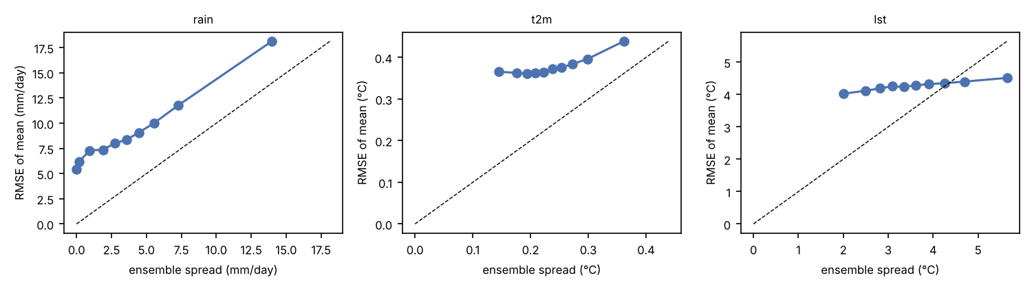
For rainfall and temperature the ensemble is under-dispersed. The spread-to-skill ratio (root-mean-square spread over RMSE of the ensemble mean) is 0.58 for rainfall, 0.64 for 2 m temperature and 0.87 for land-surface temperature, and the twelve-member envelope contains the observation on 79 % of rainfall cell-days, 66 % of temperature cell-days and 85 % of land-surface cell-days, against the 84.6 % a calibrated twelve-member ensemble would give. Figure 7 shows the binned spread-skill relation; the rainfall curve sits above the diagonal throughout.
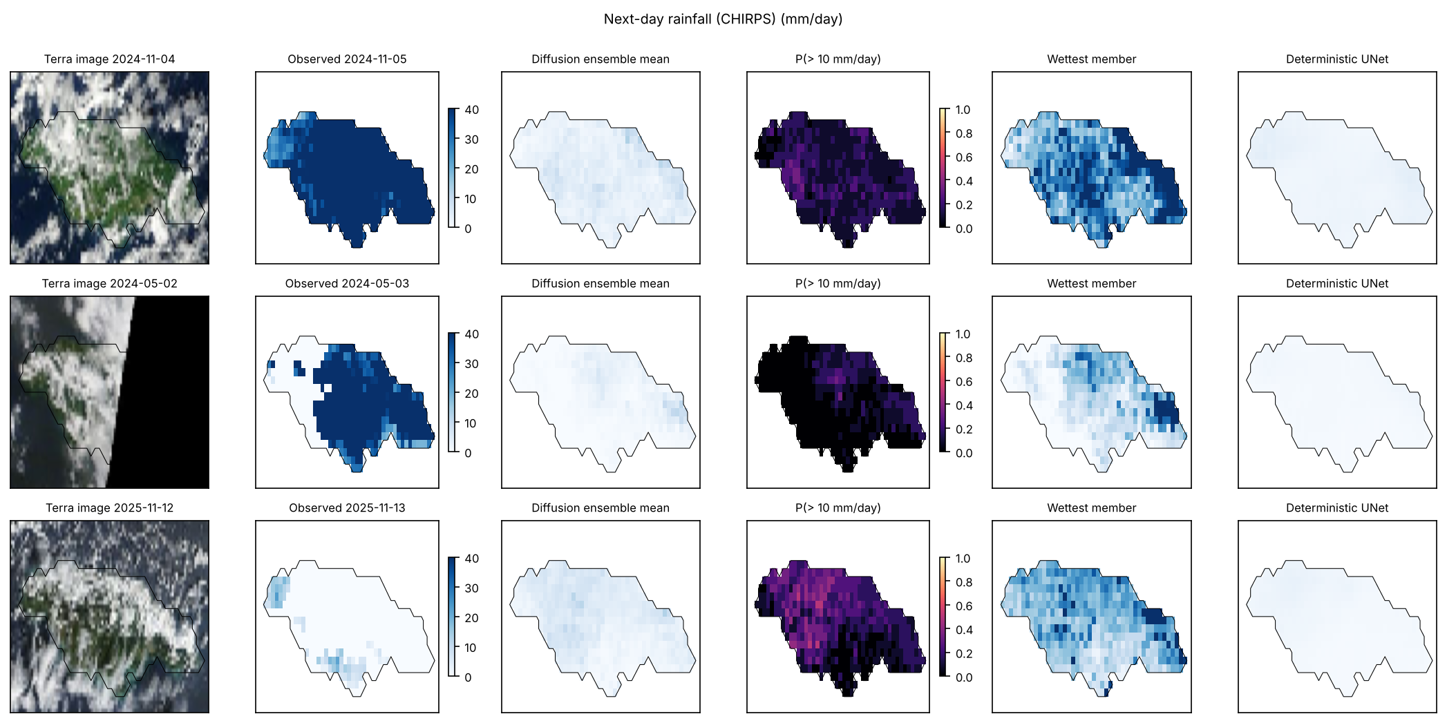
What the ensemble misses is the largest events. On the three wettest test days (Table 5) the observed island-mean rainfall was 65, 47 and 41 mm/day. The ensemble means were 3.8, 1.3 and 14.2 mm/day, and the wettest of twelve members reached 27.8, 7.3 and 42.8 mm/day. On the day after Tropical Storm Rafael’s passage (5 November 2024), when every land cell exceeded 10 mm, the ensemble gave that exceedance a mean probability of 0.125. The day before Hurricane Melissa’s landfall was the only one of the three on which the ensemble carried substantial probability (0.48), and persistence did better still because the previous day was already wet. The deterministic UNet predicted 2.1, 0.7 and 7.3 mm/day on the same three days. Nothing the model saw in one day’s imagery told it that the next day would be exceptional.
| Image day | Target day | Observed | Ensemble mean | Wettest member | P(10) | Fraction 10 | UNet |
|---|---|---|---|---|---|---|---|
| 2024-11-04 | 2024-11-05 | 64.8 | 3.8 | 27.8 | 0.125 | 1.00 | 2.1 |
| 2024-05-02 | 2024-05-03 | 46.8 | 1.3 | 7.3 | 0.048 | 0.73 | 0.7 |
| 2025-10-27 | 2025-10-28 | 41.2 | 14.2 | 42.8 | 0.477 | 1.00 | 7.3 |
What the imagery adds
Switching the imagery channels off at inference, which leaves the previous day’s fields and the season, changes little. For rainfall the ensemble with imagery has lower RMSE by 0.17 mm/day with interval and lower CRPS by 0.05 mm/day with interval . Its fractions skill scores are higher (0.325 against 0.296 at 10 mm, 0.132 against 0.104 at 25 mm), its island-mean correlation with the observations is higher (0.44 against 0.38), and its Brier skill at 10 mm is 0.208 against 0.194. For 2 m temperature the two queries are the same to three decimals, and for land-surface temperature the differences are inside their intervals. The pictures carry a small, consistent amount of next-day rainfall information and no next-day temperature information that the previous day’s field did not already hold.
Training and cost
Validation loss for the diffusion model fell through all 40 epochs (0.344 to 0.152) and the final epoch was kept. The UNet’s validation loss reached its minimum at epoch 13 of 20 (0.321) and rose afterwards; that checkpoint was kept. Training took 47 minutes for the diffusion model and 24 minutes for the UNet on two CPU cores. Generating the 730-day test ensembles with and without imagery, together with the UNet predictions, took 35 minutes. Ridge regression with the validation-chosen penalty of 1.0 fits in under a minute. A 24-day validation check of the sampler before the test run gave ensemble-mean errors of 1.32, 0.26 and 0.82 standard units for the three targets against 1.30, 0.27 and 0.96 for persistence, which is the pattern the test years then showed.
Discussion
Four findings carry the paper. A conditional diffusion model trained on 14 years of daily satellite pictures produces next-day ensembles whose probabilistic scores beat every deterministic reference tested, by 15 to 38 % in CRPS. Scored against distributions built from the observations alone, the same ensembles show no demonstrated skill: a rainfall CRPS within about 3 % of three references, on either side of them, a Brier score at 10 mm no better than the climatological frequency, and a temperature CRPS 19 % worse than dressed persistence. The ensemble mean is no better a point forecast than the simplest references. And the pictures themselves add only a little, a small rainfall gain and nothing for temperature.
The first finding is the expected consequence of generating instead of regressing. A squared-error regression in log-rain space converges to a conditional mean that almost never exceeds 10 mm in any cell. It scores well on MAE, where the many dry cell-days dominate, and badly on anything that asks where heavy rain is likely. The diffusion model’s members are individually plausible fields, so exceedance probabilities and the CRPS reward it, in line with what LDCast, PreDiff and GenCast report at their own scales (Leinonen et al. 2023; Gao et al. 2023; Price et al. 2025).
The second finding is the one a reader should carry away. Most of the gain attributed to generation in the first comparison is the gain any calibrated distribution makes over a point forecast. A Markov-chain climatology with three states and no fitted parameters has a lower rainfall CRPS than a 1.7-million-parameter network that read six satellite layers. The defensible description of the model is that it has learned the climatological distribution of Jamaican daily rainfall, conditioned weakly on the previous day, and that it represents this distribution as spatially coherent fields. The references were scored cell by cell, and the Markov-chain reference is conditioned cell by cell, so nothing in this comparison tests spatial structure. Whether coherent fields have value beyond the marginals is a question for field-valued scores, the fractions skill score or an energy or variogram score (Gneiting and Raftery 2007) computed for the references as well as the model, and that comparison has not been made.
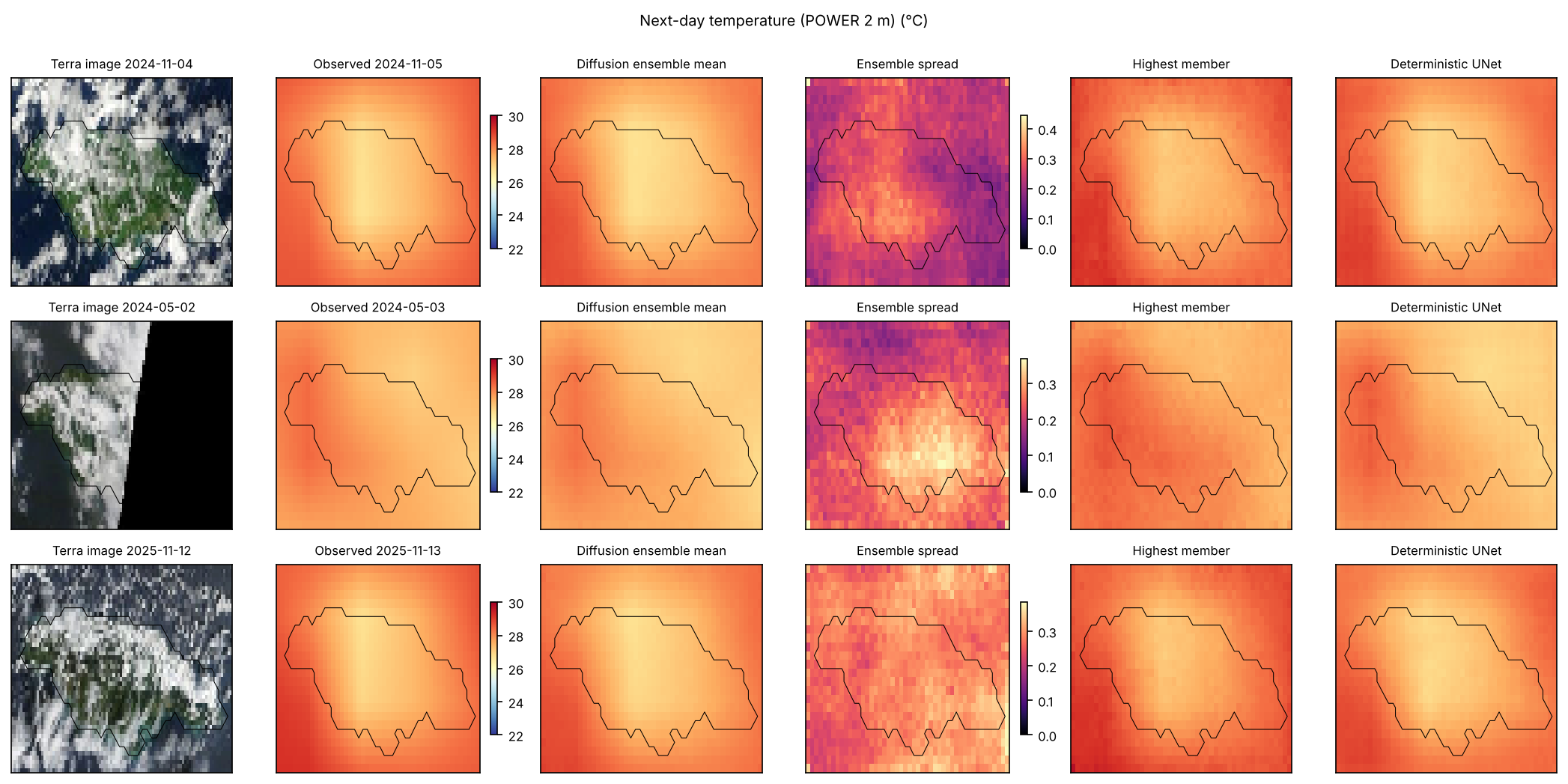
The third finding follows directly from averaging. An ensemble mean sacrifices sharpness, and on a smooth target such as interpolated 2 m temperature, persistence at 0.34 °C RMSE is hard to beat with anything.
The fourth finding is the one that matters for how satellite imagery should be used here. The six layers cover cloud, moisture, surface temperature and rain already falling, and a forecaster reads them as a picture of the atmosphere’s state at overpass time. The model extracts about a 1.5 % rainfall improvement from them and misses the three largest rain days almost completely. Several reasons are plausible and the design cannot separate them. Daytime overpasses at 10:30 and 13:30 local time say little about a system that arrives overnight; Rafael’s rain on 5 November followed a 4 November image that shows cloud but not the storm’s approach. A 24-hour step is long relative to the life of convective cells, which is why nowcasting work conditions on 10-minute geostationary imagery (Chase et al. 2025). The true-colour composites are rendered pictures, not calibrated radiances, and the palette layers were decoded through colour bins. And 5,114 training pairs contain few events of the size that was missed, so the model’s prior for an island-wide 60 mm day is weak regardless of what the picture shows.
Persistence’s fractions skill score, higher than the ensemble’s at both thresholds, points to the same gap from the other side, and so does the Markov-chain reference, which gains its edge from the previous day’s state alone. The ensemble’s exceedance probabilities are too spread out in space; where rain fell yesterday remains the single best indicator of where it falls today at this resolution. A model that combined persistence’s spatial memory with the ensemble’s calibration, through a residual formulation such as CorrDiff’s (Mardani et al. 2025) with persistence as the base, is the natural next design.
Two results are practical. The whole pipeline, from image fetch to scored ensembles, runs on public services and two CPU cores in an afternoon, and the imagery arrives as pictures that a browser could display. A regional group can reproduce it without a data-centre allocation or a satellite data licence. And the -prediction failure recorded in the methods is worth passing on. With a small model, a small dataset and a coarse sampler, the parameterisation decided whether the ensembles were usable at all, before any question about the science could be asked.
Limitations
Rainfall is scored against a satellite-and-gauge product rather than gauge truth, and the model’s skill is skill at reproducing CHIRPS, including its known underestimation of extreme totals over Jamaica. The Melissa landfall day appears in CHIRPS as a 41 mm/day island mean. The 2 m temperature target is a 0.5 ° reanalysis-based field interpolated to the grid, so the temperature task has little fine-scale content to predict. Land-surface temperature is scored only where the satellite saw the ground, which conditions the comparison on clear sky. The imagery is rendered, not radiometric, and 31 days of late 2022 are absent. The imagery ablation zeroes channels at inference on a model trained with imagery dropout; no second model was trained without pictures. The probabilistic references were added after the test scores had been seen, they are per-cell or lagged-field distributions that were not tuned, and their comparison with the model has no paired interval. Twelve members and 32 sampling steps are small for a diffusion ensemble, and one seed was run for each learned model, so run-to-run variation is unmeasured. The bootstrap intervals treat 30-day blocks of the two test years as exchangeable and are descriptive. The study is retrospective, with final products as inputs and no latency. The test years were not seen during development, and they were the only test years available, so there is no replication.
Conclusion
A conditional diffusion model can turn a day’s satellite pictures of Jamaica into a next-day ensemble of rainfall and temperature fields that beats persistence, the climatological mean, a per-pixel ridge regression and a deterministic UNet on probabilistic scores over 730 held-out days. That comparison flatters it. Against a climatological distribution, a three-state Markov-chain climatology and a lagged ensemble, its rainfall CRPS differs by , and −2.8 % in skill, its Brier score at 10 mm is no better than the climatological frequency, and for 2 m temperature dressed persistence is better by 19 %. The ensemble is under-dispersed, its mean is no better a point forecast than the simplest references, and it misses the three largest rain days of 2024 and 2025 almost entirely. Switching the imagery off costs about 1.5 % of rainfall CRPS and nothing for temperature. The findings support two requirements for the next model: it has to be scored against probabilistic references from the start, and it needs a source of information about tomorrow that once-daily pictures and yesterday’s fields do not hold. They do not support a claim of forecast skill for this one.
Data and code availability
All inputs are public, from GIBS (NASA EOSDIS), CHIRPS v2.0 (Climate Hazards Center, read through the IRI Data Library) and NASA POWER. The package accompanying this draft holds the fetch and decoding scripts with per-request manifests and SHA-256 hashes, the assembled day-pair dataset, the model and training code, the trained weights, the ensemble and baseline prediction files, the scored results and every figure and animation. The probabilistic references are computed by prob_refs.py from the re-fetched targets, with their own manifest of source hashes, and written to prob_refs_test.json. The script reproduces the archived deterministic scores as its control before it scores anything new.