Keywords: Jamaica; CHIRPS; precipitation downscaling; hard constraints; conservation; physics-informed learning; driver bias.
1 Introduction
A rainfall field can be internally consistent without being accurate. On an island with sharp spatial gradients and few verifying gauges, those two properties have to be measured separately. This paper measures them for one restricted, testable task: the allocation of a known coarse monthly total to finer cells while preserving that total. Two questions follow. Does the constraint improve an otherwise matched network? And does the network add anything over a transparent seasonal baseline that conserves the same total?
A third question comes from the way such a component would be used. A downscaler trained on retrospectively analysed rainfall will later be driven by a forecast, a reanalysis or a climate model. Exact consistency with a wrong coarse total transmits the aggregate error into the fine-scale estimate. I quantify that transmission with controlled perturbations of the real coarse fields and with a driver that predates the target month, and I give the elementary bound that explains the result.
The contribution is an executed regional benchmark, with trained models, held-out reconstructions, numerical checks and counter-examples, and with its negative findings disclosed. It does not introduce a conserving architecture; exact downscaling constraints exist [1, 2], and so does neural rainfall modelling in Jamaica [3] and climatology-weighted disaggregation [4]. It does not test geographic transfer, which benchmarks such as RainShift [5] address.
2 Related work
Physics-informed learning spans residual-equation models [6, 7] and conservative domain-decomposition methods [8]; both impose more than the area-mean condition tested here. Optimisation failures in such networks [9] are a warning against reading a low constraint residual as evidence of skill. Jamaican CHIRPS analyses supply local precedent for the record [10], Caribbean gauge comparisons show why gridded products need regional assessment [11], and resolution-dependent studies of the region motivate explicit treatment of small islands [12, 13, 14]. Greater Antilles extreme-rainfall work gives the regional context that a monthly reconstruction cannot address [15].
Learned multiresolution downscaling [16] and generative downscaling [17, 18] represent unresolved variability in ways this deterministic design does not try to. Process-informed bias correction [19] is the relevant literature whenever the driver differs systematically from the target, which is the subject of Section 5.
3 Data and design
3.1 CHIRPS fields, cells and parents
Monthly CHIRPS v2 fields [20] for January 2000 to December 2025 were downloaded from the Central America and Caribbean archive; all 312 source files have recorded URLs and SHA-256 hashes. CHIRPS blends satellite information with station observations, so the experiment uses a satellite-gauge product rather than raw imagery. A window of roughly 78.5 °W to 76.1 °W and 17.5 °N to 18.7 °N and a geoBoundaries Jamaica polygon identify land cells by centre inclusion. Of 374 valid land cells, 360 remain after requiring at least four represented cells per parent, giving 29 parents at 0.20 ° spacing over 0.05 ° children. Coastal cells count as whole cells, with fractional coastline left unresolved.
With on retained children of parent and zero elsewhere, the observed coarse depth is (1) The principal task is conditional spatial downscaling. The model receives the target month’s observed and allocates it, so nothing here is a month-ahead forecast. Fitting uses 2000–2017 (216 months, 6,264 parent-months), checkpoint selection 2018–2021 (48 months) and assessment 2022–2025 (48 months, 17,280 cell-months that are not treated as independent). The same locations occur in every period, so temporal blocking [21] addresses one dependence and leaves spatial transfer untested.
3.2 Matched networks and the three output rules
Each network has two fully connected ReLU layers of width 64 and 16 output units, 5,968 parameters. Its 11 predictors are log-transformed coarse rainfall at the parent and its four neighbours (a missing or ocean neighbour is replaced by the parent), sine and cosine of the first two annual harmonics, and longitude and latitude. Terrain, humidity, wind, temperature and lateral fluxes are absent. With , the free output and the exactly conserving output are (2) The weighted mean of equals by construction. This is a cross-scale consistency condition; it does not close a moisture budget, solve an equation or enforce flux continuity between parents. The soft model uses with the loss (3) with the training-target root-mean-square depth; free and hard models use the first term only. Adam runs at learning rate with weight decay on shuffled batches of at most 256 parent-months for 200 epochs; validation RMSE at epoch 1 and every fifth epoch selects the checkpoint. Seeds 11, 29 and 47 share initial weights and shuffles across model types. Penalties 0.1, 1 and 10 were compared on mean validation RMSE and 0.1 was selected in every record-length setting. Predictions average the three seeds and every individual fit is retained.
3.3 Baselines, scores and numerical checks
Uniform allocation gives every child . Seasonal spatial allocation takes each child’s training-period mean for the calendar month, normalises it by its parent’s weighted mean and scales the ratio by the supplied ; it conserves the same volume, uses no validation or test targets, and holds a separate climatological pattern for every month, which makes it a substantive comparator for a spatially shared network.
Area-weighted RMSE, MAE and signed bias measure agreement with CHIRPS; the conservation residual is . Paired circular month-block bootstraps use 2,000 resamples at block lengths of 3 and 12 months with complete spatial fields carried in each sampled month. The intervals describe variability of paired differences for fixed fitted ensembles and exclude reference-product uncertainty and retraining. Every serialised prediction group is rescored with a separate float64 accumulation; hard residuals are checked against a 0.002 mm tolerance; and a deliberately mis-normalised prediction (a conserving field multiplied by 1.05) must be rejected by the validator. These checks establish numerical consistency of the saved experiment. The design was specified before the fits, but earlier exploratory work had inspected overlapping CHIRPS years, so the assessment is retrospective rather than a pristine holdout.
4 Results: conservation and allocation
4.1 Primary comparison
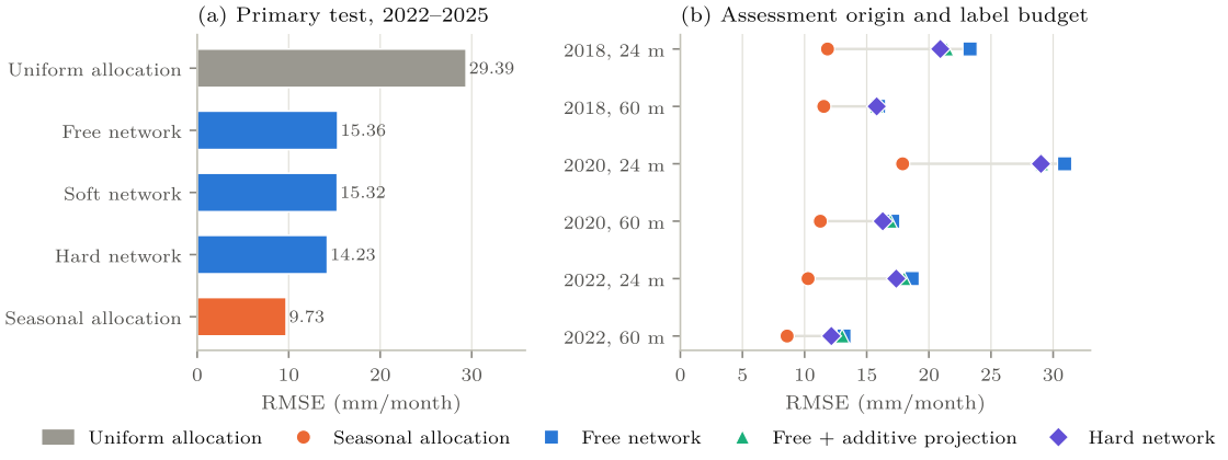
Exact conservation lowers ensemble RMSE from 15.36 to 14.23 mm/month, a difference of 1.14 mm/month or 7.4 %, with a 12-month-block interval of and a 3-month-block interval of (Table 1). The selected soft penalty moves RMSE by only −0.05 mm/month. A small penalty permits coarse-mean errors, so the soft model’s largest residual, 16.83 mm/month, is close to the free model’s 16.91, where the hard model’s is 0.00006 mm/month.
Seasonal allocation reaches 9.73 mm/month. The hard model is 4.49 mm/month worse, which is 32 % of its own score, with a 12-month-block interval of . A comparison restricted to uniform interpolation (29.39 mm/month) would overstate the network’s value by a wide margin. The month-specific climatological pattern gives lower error than the tested neural representation.
| Model | RMSE | MAE | Bias | Max. residual |
|---|---|---|---|---|
| Uniform allocation | 29.39 | 18.04 | 0.00 | 0.00000 |
| Seasonal allocation | 9.73 | 6.03 | 0.00 | 0.00001 |
| Free network | 15.36 | 9.83 | 0.13 | 16.90736 |
| Soft network () | 15.32 | 9.78 | 0.03 | 16.82706 |
| Hard network | 14.23 | 9.10 | 0.00 | 0.00006 |
4.2 Training budget
Of the 45 primary fits, 34 selected epoch 200, the last permitted. A documented post-score diagnostic reran the full-record free and hard models for 1,000 epochs with the same seeds and checkpoint rule; ensemble RMSE fell to 13.52 and 12.57 mm/month. The 200-epoch scores remain primary and the longer runs are exploratory. They show budget sensitivity rather than convergence, and the ordering against seasonal allocation survives them. The label-budget experiment below uses early stopping for up to 1,000 epochs and retains the same ordering.
4.3 Post hoc projection controls
A final correction can improve squared error without learning a better fine-scale pattern. Two post hoc controls therefore act on the saved free-model predictions within each parent: additive projection and multiplicative normalisation . Both use exactly the coarse information the hard network uses; both were specified after the original scores. Table 2 gives the results for the 18-year fit and for two restricted fitting histories (2015–2017 and 2017 alone, each still with 48 validation months). Additive projection removes the coarse-mean error contribution exactly, up to accumulation tolerance, yet for the 18-year ensemble the hard-minus-additive difference is −0.992 mm/month with a 12-month-block interval of (5,000 resamples, seed 20261007), and hard-minus-multiplicative is with . Training under the constraint does more than projecting after the fact, and the gap to seasonal allocation remains in every row.
| Fitting years | Free | Additive | Multiplicative | Hard | Seasonal |
|---|---|---|---|---|---|
| 18 (2000–2017) | 15.362 | 15.217 | 15.248 | 14.226 | 9.733 |
| 3 (2015–2017) | 17.766 | 17.459 | 17.482 | 16.426 | 9.606 |
| 1 (2017) | 20.791 | 20.108 | 20.116 | 19.068 | 11.375 |
4.4 Origin windows and label budgets
A post-review experiment budgets fitting and validation labels jointly across three chronological windows. For assessment origins 2018, 2020 and 2022, the preceding calendar year is validation and the following 24 months are assessment; a 24-month budget supplies 12 fitting plus 12 validation months and a 60-month budget 48 plus 12. The same seeds and matched free and hard architectures train for up to 1,000 epochs with validation every five epochs and a 150-epoch patience; the checkpoint minimises validation RMSE and no test score enters any choice. The seasonal comparator uses fitting labels only. This adds 36 fits, of which 21 reach the epoch cap.
The hard ensemble beats the free ensemble in six of six origin-budget comparisons; seasonal allocation beats the hard ensemble in six of six; hard training beats additive projection in five of six, the exception being the 2018 origin with a 60-month budget (Table 3). Fitting periods overlap and the same locations recur, so the six rows are descriptive comparisons, not six replications, and no pooled significance is claimed.
| Origin | Budget (months) | Seasonal | Free | Additive | Hard |
|---|---|---|---|---|---|
| 2018 | 24 | 11.844 | 23.314 | 21.432 | 20.920 |
| 2018 | 60 | 11.546 | 15.951 | 15.790 | 15.799 |
| 2020 | 24 | 17.890 | 30.926 | 29.092 | 29.018 |
| 2020 | 60 | 11.268 | 17.093 | 16.898 | 16.289 |
| 2022 | 24 | 10.279 | 18.652 | 18.003 | 17.374 |
| 2022 | 60 | 8.592 | 13.171 | 13.027 | 12.153 |
4.5 Station comparison
NOAA Global Summary of the Day records [22] for Norman Manley International (78397099999) and Sangster International (78388099999) were screened strictly: daily precipitation in inches converted to millimetres, 99.99 sentinels and incomplete-period flags excluded, only D, F and G report types accepted, and a monthly total admitted only when every calendar day qualifies. No Norman Manley test month passes; nine Sangster months do, at a cell 3.42 km from the gauge.
At Sangster the CHIRPS reference cell itself has RMSE 126.02 mm/month against the gauge. The free network has 93.67, the soft 93.65, the hard 99.36 and seasonal allocation 124.50. The within-CHIRPS ranking does not reproduce at the station, where the hard network is less accurate than the free one and the two models that reproduce CHIRPS most faithfully (seasonal allocation and the reference cell) do worst. Nine irregular coastal months cannot adjudicate between a support mismatch, a reference-product error and a real difference, and station independence from CHIRPS gauge assimilation has not been established. The station comparison illustrates the risk that a model fitted to a gridded product also reproduces its errors.
5 Results: driver error
5.1 Controlled multiplicative perturbations and the aggregation floor
For each held-out month the five coarse predictors and the output scaling depth are multiplied by before the log transform; harmonics and coordinates are unchanged, the target field is the original CHIRPS observation, and the models are evaluated at their validation-selected checkpoints without refitting. Let be the true area mean of within a parent, the supplied driver, and its weighted mean. For an exactly conserving prediction , and the weighted variance identity gives (4) Summed with parent-area weights and averaged over time this is an RMSE floor from the coarse errors alone. It is elementary and not a theorem of this paper; it is a diagnostic that no refinement of the within-parent pattern can lower while exact consistency with an erroneous driver is kept, and the serialised predictions were checked against it in every scenario.
At the hard model’s RMSE is 35.27 and 34.87 mm/month against a floor of 31.67; at it is 21.59 and 21.27 against a floor of 15.83 (Table 4). Equation 4 says the two parts add in quadrature, and they do. Removing the floor in quadrature leaves 14.2 to 15.5 mm/month in all four scenarios, close to the unperturbed 14.23. The perturbation adds parent-mean error and leaves the within-parent pattern error almost unchanged. The free and soft models do not repair the imposed bias. Their errors stay close to the hard model’s, so permitting a consistency residual does not by itself make an estimator identify and correct an unknown driver bias. Neither was trained on a corrected-driver task, so this is not evidence against learned bias correction in general. Seasonal allocation is better than every network under all four factors.
| Coarse bias | Free | Soft | Hard | Seasonal | Floor |
|---|---|---|---|---|---|
| 20 % | 35.70 | 35.83 | 35.27 | 33.48 | 31.67 |
| 10 % | 22.31 | 22.43 | 21.59 | 18.68 | 15.83 |
| 10 % | 22.12 | 21.89 | 21.27 | 18.93 | 15.83 |
| 20 % | 35.48 | 35.17 | 34.87 | 33.76 | 31.67 |
5.2 Drivers available before the target month
A seasonal driver replaces the coarse predictors and scaling depth with each calendar month’s 2000–2017 coarse average; a lag-12 driver uses the same calendar month of the preceding year. Calendar features are kept. The networks were trained under contemporaneous conditioning, so this distribution shift is deliberate and limits interpretation to dependence on driver quality.
Hard-model RMSE rises from 14.23 to 84.49 mm/month with the seasonal driver and to 109.84 with lag-12 input; seasonal allocation gives 83.97 and 109.56, and uniform allocation 87.12 and 111.16 (Table 5). The differences between allocation methods are small beside the loss of contemporaneous coarse information. The hard network still meets its supplied totals in every scenario, with a largest residual below 0.0002 mm/month. That success is agreement with the input; it says nothing about the unknown outcome. A paper reporting the 14.23 mm/month conditional score as predictive skill would misdescribe the experiment.
| Driver | Uniform | Seasonal | Free | Soft | Hard |
|---|---|---|---|---|---|
| Seasonal (2000–2017 mean) | 87.12 | 83.97 | 84.58 | 84.56 | 84.49 |
| Lag-12 (previous year) | 111.16 | 109.56 | 109.84 | 109.76 | 109.84 |
6 Discussion
Exact area normalisation improves this network’s conditional reconstruction and makes its aggregation error negligible, and the gain survives projection controls, a longer training budget and six further windows. The seasonal comparator changes what that property is worth. A climatological pattern scaled by the same observed total has 4.49 mm/month lower RMSE on the primary test. It also has lower RMSE in the additional within-CHIRPS comparisons. The experiment supports retaining a conserving layer as a component; it does not justify replacing a well-performing climatological allocation with this model.
The result is specific to monthly CHIRPS reconstruction on a small, repeatedly observed island. Month aggregation suppresses sub-daily variability, and an 18-year record lets the network and the baseline encode a stable spatial climatology. Coordinates as predictors encode recurring location patterns, which is appropriate within the island and says nothing about transfer. Wet-day occurrence, storm timing, flood thresholds, calibrated uncertainty and transfer off the island are all outside what this benchmark can show.
The station comparison is consequential. A network trained to reproduce one gridded product may be rewarded for reproducing that product’s errors, and a smoother model may score better at a gauge without reconstructing the field any better. Nine months cannot separate these. More quality-controlled gauges with documented assimilation status would be worth more than a larger network.
The driver analysis supplies an acceptance criterion. If a proposed allocation method claims exact consistency on the same cells and reports error below the driver’s unavoidable aggregation error, then some support, weight, target or conservation definition differs, and a data and metric audit should precede any skill claim. For an operational model the coarse total can be corrected before downscaling or treated probabilistically; either choice changes what is conserved and should be stated. Hard consistency with a bias-corrected driver conserves the corrected total rather than the original model output.
7 Design of a real-driver study
The four uniform multipliers do not span spatially varying bias, seasonal drift, displaced storms or errors coupled to intensity. A separate study should identify a coarse precipitation source and its release latency, align spatial support and accumulation periods, estimate bias correction from development data only, and train and assess raw-driver conservation, corrected-driver conservation, a tuned soft constraint, an unconstrained alternative and seasonal allocation under the same issuance-available information. Evaluation should separate parent-mean error from within-parent anomaly error and use gauges whose assimilation status is known. Atmospheric-state predictors from ERA5 [23], distinguished from ERA5-Land surface fields [24], a second product such as IMERG [25] and SRTM elevation [26] are the natural additions; none was used here. The present component has no learned lateral interface, overlapping solver or moisture transport; a moisture-budget test needs water-vapour storage, evaporation and transport on compatible supports, which the conservation residual used here cannot stand in for.
8 Conclusion
Exact volume conservation improves a matched neural downscaler over Jamaica by 7.4 % in RMSE and makes its aggregation error negligible, and the gain survives projection controls, a longer training budget and six further windows. Seasonal climatological allocation has 32 % lower RMSE on the primary test and remains more accurate in the additional within-CHIRPS comparisons. When the coarse driver is wrong, exact consistency imposes an aggregate-error floor that no within-parent refinement can lower, and a driver that predates the target month raises error roughly six to eight times. The findings support keeping a conserving layer available and reporting driver accuracy alongside any conservation residual. They do not support replacing a climatological allocation with this network, and they do not measure forecast skill.
Data and code availability
The experiment archive holds acquisition scripts, source hashes, model-ready arrays, checkpoints, station quality-control records, the total-label-budget protocol with its 36 checkpoints and validation histories, seed-level and ensemble predictions, exact score tables and the projection-control analysis. The driver-sensitivity analysis reuses the fitted models, so it adds no independent replication. CHIRPS v2 and the NOAA Global Summary of the Day are public; the archive is held by the author and is available on request. It was not re-executed for this draft, so the numbers here are those of the archived reports rather than an independent replication.
References
[1] Paula Harder, Alex Hernandez-Garcia, Venkatesh Ramesh, Qidong Yang, Prasanna Sattegeri, Daniela Szwarcman, Campbell Watson, and David Rolnick. Hard-constrained deep learning for climate downscaling. Journal of Machine Learning Research, 24 (365): 1–40, 2023. https://www.jmlr.org/papers/v24/23-0158.html.
[2] Tom Beucler, Michael Pritchard, Stephan Rasp, Jordan Ott, Pierre Baldi, and Pierre Gentine. Enforcing analytic constraints in neural networks emulating physical systems. Physical Review Letters, 126 (9): 098302, 2021. doi: 10.1103/PhysRevLett.126.098302.
[3] Christina P. Burgess, Michael A. Taylor, Tannecia Stephenson, and Arpita Mandal. Frequency analysis, infilling and trends for extreme precipitation for Jamaica (1895–2100). Journal of Hydrology: Regional Studies, 3: 424–443, 2015. doi: 10.1016/j.ejrh.2014.10.004.
[4] Silvia Terzago, Elisa Palazzi, and Jost von Hardenberg. Stochastic downscaling of precipitation in complex orography: a simple method to reproduce a realistic fine-scale climatology. Natural Hazards and Earth System Sciences, 18: 2825–2840, 2018. doi: 10.5194/nhess-18-2825-2018.
[5] Paula Harder et al. RainShift: A benchmark for precipitation downscaling across geographies. arXiv:2507.04930, 2025.
[6] Maziar Raissi, Paris Perdikaris, and George Em Karniadakis. Physics-informed neural networks: A deep learning framework for solving forward and inverse problems involving nonlinear partial differential equations. Journal of Computational Physics, 378: 686–707, 2019. doi: 10.1016/j.jcp.2018.10.045.
[7] George Em Karniadakis, Ioannis G. Kevrekidis, Lu Lu, Paris Perdikaris, Sifan Wang, and Liu Yang. Physics-informed machine learning. Nature Reviews Physics, 3: 422–440, 2021. doi: 10.1038/s42254-021-00314-5.
[8] Ameya D. Jagtap, Ehsan Kharazmi, and George Em Karniadakis. Conservative physics-informed neural networks on discrete domains for conservation laws: Applications to forward and inverse problems. Computer Methods in Applied Mechanics and Engineering, 365: 113028, 2020. doi: 10.1016/j.cma.2020.113028.
[9] Aditi S. Krishnapriyan, Amir Gholami, Shandian Zhe, Robert M. Kirby, and Michael W. Mahoney. Characterizing possible failure modes in physics-informed neural networks. In Advances in Neural Information Processing Systems 34 (NeurIPS), 2021. arXiv:2109.01050.
[10] C. Avalon Cullen and Rafea Al Suhili. Assessing rainfall variability in Jamaica using CHIRPS: Techniques and measures for persistence, long and short-term trends. Geographies, 3 (2): 375–397, 2023. doi: 10.3390/geographies3020020.
[11] Abel Centella-Artola, Arnoldo Bezanilla-Morlot, Michael A. Taylor, Dimitris A. Herrera, Daniel Martín-Serrano, Maibys Sierra-Lorenzo, Alejandro Vichot-Llano, Jesús Cabrales-Infante, Jayaka D. Campbell, and Tannecia S. Stephenson. Evaluation of sixteen gridded precipitation datasets over the Caribbean region using gauge observations. Atmosphere, 11 (12): 1334, 2020. doi: 10.3390/atmos11121334.
[12] Mark R. Jury. Resolution-dependent perspectives on Caribbean hydro-climate change. Hydrology, 7 (4): 93, 2020. doi: 10.3390/hydrology7040093.
[13] Philippe Cantet, Michel Déqué, Philippe Palany, and Jean-Louis Maridet. The importance of using a high-resolution model to study the climate change on small islands: the Lesser Antilles case. Tellus A: Dynamic Meteorology and Oceanography, 66: 24065, 2014. doi: 10.3402/tellusa.v66.24065.
[14] Jayaka D. Campbell, Michael A. Taylor, Arnoldo Bezanilla-Morlot, Tannecia S. Stephenson, Abel Centella-Artola, Leonardo A. Clarke, and Kimberly A. Stephenson. Generating projections for the Caribbean at 1.5, 2.0 and 2.5 C from a high-resolution ensemble. Atmosphere, 12 (3): 328, 2021. doi: 10.3390/atmos12030328.
[15] Carlo Destouches, Arona Diedhiou, Sandrine Anquetin, Benoit Chanzy, Adermus Joseph, Nathan Pierre, and Adrien Dumont. Changes in extreme precipitation patterns over the Greater Antilles and teleconnection with large-scale sea surface temperature. Earth System Dynamics, 16: 497–530, 2025. doi: 10.5194/esd-16-497-2025.
[16] Jiali Wang, Zhengchun Liu, Ian Foster, Won Chang, Rajkumar Kettimuthu, and V. Rao Kotamarthi. Fast and accurate learned multiresolution dynamical downscaling for precipitation. Geoscientific Model Development, 14: 6355–6372, 2021. doi: 10.5194/gmd-14-6355-2021.
[17] Lucy Harris, Andrew T. T. McRae, Matthew Chantry, Peter D. Dueben, and Tim N. Palmer. A generative deep learning approach to stochastic downscaling of precipitation forecasts. Journal of Advances in Modeling Earth Systems, 14 (10): e2022MS003120, 2022. doi: 10.1029/2022MS003120.
[18] Michael Aich, Philipp Hess, Baoxiang Pan, Sebastian Bathiany, Yu Huang, and Niklas Boers. Conditional diffusion models for downscaling and bias correction of Earth system model precipitation. arXiv:2404.14416, 2024.
[19] Douglas Maraun, Theodore G. Shepherd, Martin Widmann, Giuseppe Zappa, Daniel Walton, José M. Gutiérrez, Stefan Hagemann, Ingo Richter, Pedro M. M. Soares, Alex Hall, and Linda O. Mearns. Towards process-informed bias correction of climate change simulations. Nature Climate Change, 7: 764–773, 2017. doi: 10.1038/nclimate3418.
[20] Chris Funk, Pete Peterson, Martin Landsfeld, Diego Pedreros, James Verdin, Shraddhanand Shukla, Gregory Husak, James Rowland, Laura Harrison, Andrew Hoell, and Joel Michaelsen. The climate hazards infrared precipitation with stations: a new environmental record for monitoring extremes. Scientific Data, 2: 150066, 2015. doi: 10.1038/sdata.2015.66.
[21] David R. Roberts, Volker Bahn, Simone Ciuti, Mark S. Boyce, Jane Elith, Gurutzeta Guillera-Arroita, Severin Hauenstein, José J. Lahoz-Monfort, Boris Schröder, Wilfried Thuiller, David I. Warton, Brendan A. Wintle, Florian Hartig, and Carsten F. Dormann. Cross-validation strategies for data with temporal, spatial, hierarchical, or phylogenetic structure. Ecography, 40 (8): 913–929, 2017. doi: 10.1111/ecog.02881.
[22] NOAA National Centers for Environmental Information. Global summary of the day: data archive and precipitation documentation. https://www.ncei.noaa.gov/data/global-summary-of-the-day/, 2026. Accessed 6 October 2026.
[23] Hans Hersbach, Bill Bell, Paul Berrisford, et al. The ERA5 global reanalysis. Quarterly Journal of the Royal Meteorological Society, 146 (730): 1999–2049, 2020. doi: 10.1002/qj.3803.
[24] Joaquín Muñoz-Sabater, Emanuel Dutra, Anna Agustí-Panareda, et al. ERA5-Land: a state-of-the-art global reanalysis dataset for land applications. Earth System Science Data, 13: 4349–4383, 2021. doi: 10.5194/essd-13-4349-2021.
[25] George J. Huffman, David T. Bolvin, Dan Braithwaite, Kuo-Lin Hsu, Robert J. Joyce, Christopher Kidd, Eric J. Nelkin, Soroosh Sorooshian, Erich F. Stocker, Jackson Tan, David B. Wolff, and Pingping Xie. Integrated multi-satellite retrievals for the Global Precipitation Measurement (GPM) mission (IMERG). In Satellite Precipitation Measurement, volume 67 of Advances in Global Change Research. Springer, 2020. doi: 10.1007/978-3-030-24568-9_19.
[26] Tom G. Farr, Paul A. Rosen, Edward Caro, et al. The Shuttle Radar Topography Mission. Reviews of Geophysics, 45 (2): RG2004, 2007. doi: 10.1029/2005RG000183.