1. Introduction
Satellite surface-temperature maps can describe the thermal pattern of roofs, roads, bare ground and vegetation within an urban study region. Their physical interpretation differs from that of a weather-station air-temperature record. The question addressed by this methods note is how the supplied Landsat composites represent spatial and seasonal surface-temperature patterns in the intended Kingston Parish study area. The retained source is Adrian Dunkley’s Explanation of the Temperature Mapping and Analysis, dated 22 June 2026, together with three display rasters [1].
The source describes a mapping workflow rather than an inferential comparison with independent measurements. This edition therefore reports the available outputs, distinguishes the stated processing from settings not preserved in the note, and sets out what would be required to reproduce and quantify the seasonal comparison. It does not estimate air temperature, human heat exposure or the causal effect of land cover.
2. Data and methods
2.1 Study area and thermal product
The documented workflow selects Landsat 8 and Landsat 9 Collection 2 Level 2 images covering the study area and clips them to an administrative boundary. The source intends this to represent Kingston Parish but warns that some boundary datasets may instead identify Kingston and St. Andrew together. The exact polygon and administrative dataset are not established by the retained note; the area is consequently described as the supplied Kingston study area.
The source uses the surface-temperature product derived from thermal infrared observations. USGS describes this product as a measure of Earth’s surface temperature [2]. Landsat 8–9 thermal bands are acquired at 100 m and resampled to a 30 m grid [3]. The original note’s description of native 30 m thermal resolution is corrected here. Its 10 m export setting is a presentation scale, not independent thermal detail at 10 m.
2.2 Observation windows
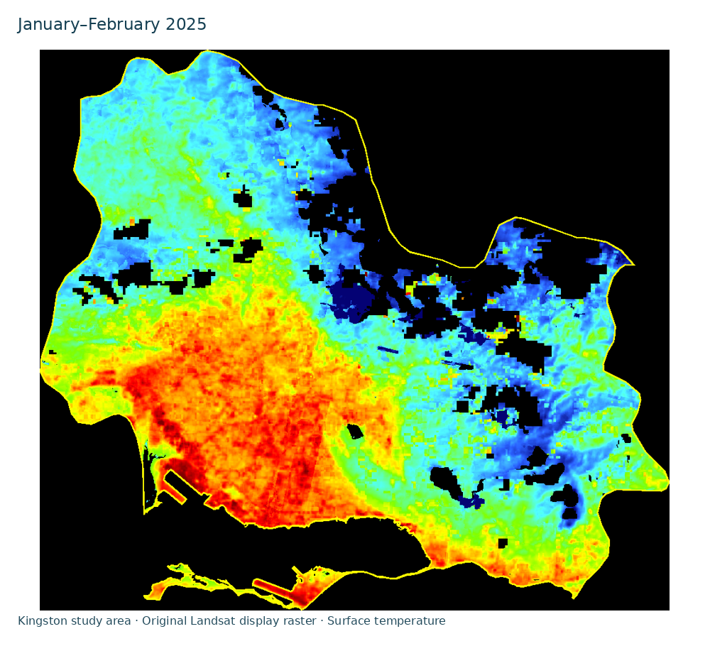
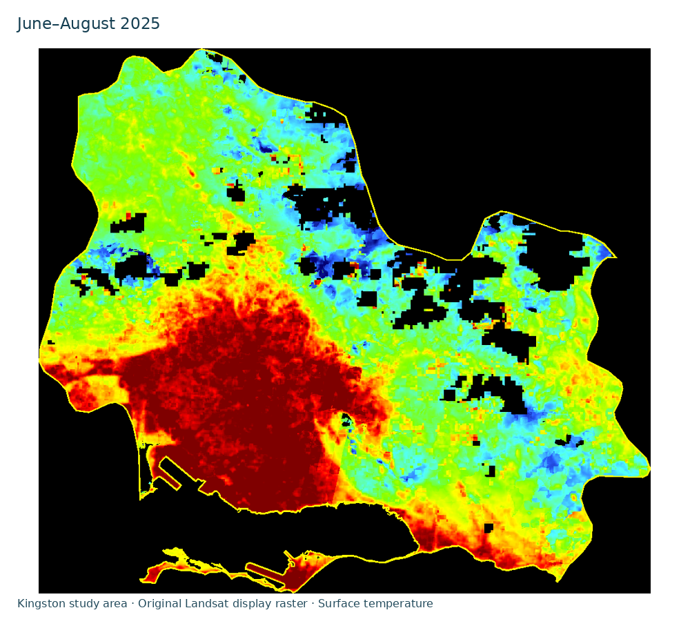
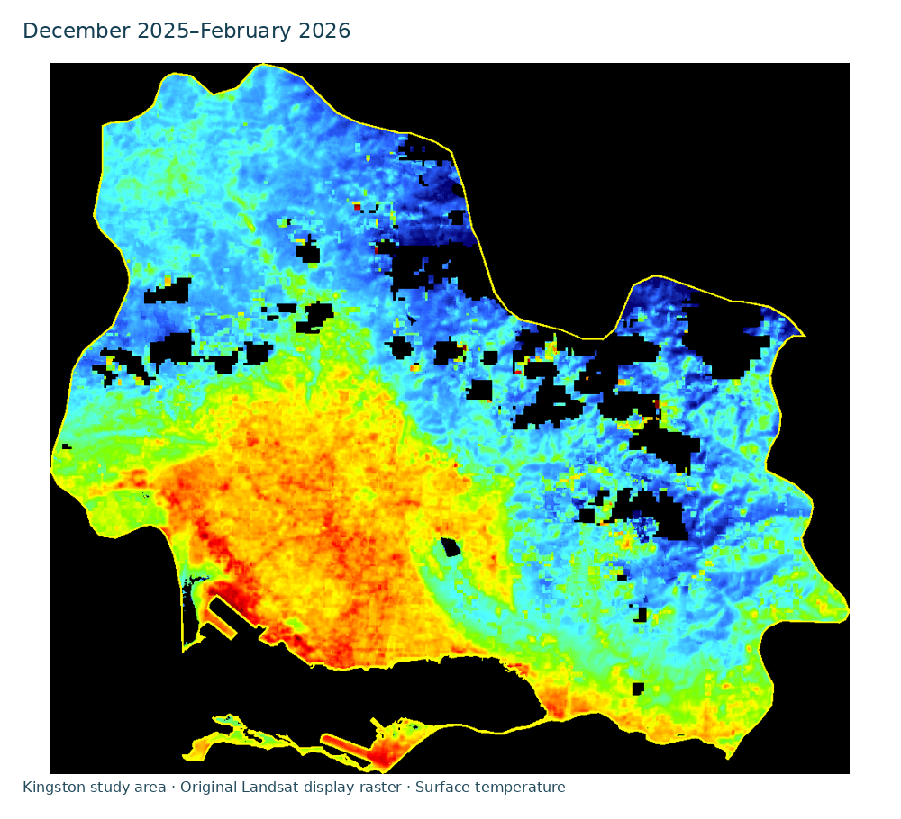
The beginning-of-year composite covers January–February 2025; the summer composite covers June–August 2025; and the winter composite covers December 2025–February 2026. The winter window extends into the following year and is not a December-only estimate. The source also describes monthly frames from January 2025 through February 2026. Only the three seasonal exports are retained for this web edition, so the animation below cycles between those composites rather than reconstructing a missing monthly sequence.
2.3 Processing and missing observations
According to the source, images were filtered by date and location; clouds, cloud shadows, cirrus, snow, fill pixels and water pixels were masked; thermal values were converted to degrees Celsius; and available images were combined within each period. The note does not preserve the collection identifiers, scene list, mask bit settings, numerical conversion implementation or composite reducer. These details should be recovered from the original code before claiming an independently reproduced workflow.
The source states that nearby valid pixels were used to fill gaps for visualisation. Interpolated values should remain distinguishable from observed values in any quantitative analysis. The retained RGB images preserve display colours, boundaries and masked regions, but they do not provide the numerical arrays or valid-observation counts required to calculate temperature statistics. No numerical temperature is inferred from an RGB colour in this edition.
2.4 Display interpretation
The source describes a scale progressing from dark blue, around 20 °C or cooler, through blue and cyan in the 20s, green near the upper 20s to low 30s, yellow and orange in the 30s, and red or dark red near 38–42 °C and above. These are descriptions of the original display scale, not newly calculated minima, maxima or area means. Black background or masked areas are not measured cold surfaces.
3. Results: retained seasonal visualisations
The available result is a set of three seasonal display maps. They allow the reader to inspect the spatial arrangement of the supplied colours and to compare the displayed periods. The original note describes warmer-colour areas as possible built-up heat hotspots and cooler-colour areas as possible vegetated or shaded locations. Those interpretations are hypotheses about land cover: no matched land-cover classification, independent temperature measurements or significance test is supplied. A quantitative ranking of seasons or neighbourhoods is therefore not reported.
4. Discussion
The maps are useful for communicating how a thermal satellite product differs from a familiar air-temperature forecast. They also show why the measurement scale and display scale must be reported separately. Resampling can make a boundary or colour field appear smoother without adding independent observations. A visually continuous map can similarly conceal interpolation across areas where no acceptable observation was retained.
A reproducible seasonal comparison would first confirm the geographic boundary and recover the original temperature rasters and processing code. It would report the number and dates of valid observations, the compositing rule and the fraction of each result that was interpolated or missing. Comparisons could then use common spatial support and explicit uncertainty. Explaining an apparent warm area would additionally require matched land-cover evidence and, for claims about air temperature or exposure, appropriate independent measurements.
5. Limitations
The retained evidence is a descriptive note and rendered images. It does not establish numerical seasonal differences, statistical significance, the magnitude of a neighbourhood heat island or a measured effect on people. The administrative boundary remains uncertain, and the source does not specify all processing choices. Cloud masking and differing observation availability can change which surfaces contribute to a composite. Interpolated display pixels cannot replace the original observations in a scientific measurement.
6. Conclusion
The preserved Landsat exports document the intended seasonal mapping exercise and its visual presentation. Their defensible use is inspection of displayed surface-temperature patterns within the supplied boundary. A publication-level quantitative study requires recovery and verification of the original arrays, sampling and processing decisions before new temperature comparisons are made.
Data and source availability
The web page retains the three seasonal display rasters and a sequence made from those rasters. The original methods note remains in the research source archive. The numerical temperature arrays, original processing code and complete acquisition record were not available for this editorial reconstruction. No new experimental run, funding, ethical approval or institutional endorsement is asserted.
References
- Dunkley, A. (2026). Explanation of the Temperature Mapping and Analysis. Author-supplied methods note, 22 June, and three accompanying Landsat display rasters. This academic edition preserves the reported workflow and records the limitations of the retained evidence.
- US Geological Survey. Landsat Surface Temperature. Official product description, inspected 14 November 2026.
- US Geological Survey. What are the band designations for the Landsat satellites? Landsat 8–9 thermal acquisition and resampling specifications, inspected 14 November 2026.