Decision and contribution
The question is whether a transparent, pre-season scenario calculation can expose the trade-off between water security and its cost without using the season’s future rainfall to select a plan. The contribution at this stage is an executable framework, an information-cutoff test and a proposed validation design. The scientific comparison separates physical consistency, predictive error and practical decision value.
The intended user is a grower or extension adviser deciding when to establish a crop and whether irrigation is affordable. On 1 March, the example considers 1 April, 15 April and 1 May establishment dates. This allows 31–61 days for nursery work, land preparation, input ordering and water arrangements. These lead times are design assumptions to be checked with farmers. Tomato and watermelon are relevant crops in St Elizabeth’s official production materials [5], [6]; their presence does not establish the suitability of the sampled point for either crop.
Each crop is assessed separately. A fixed 1 April rainfed plan is the baseline for that crop. It is a predeclared comparator, not a claim about normal local practice. Choosing a later date may change prices, labour availability and the next crop cycle. Those effects are not modelled, so the selected date is not an operational recommendation.
Related work and the scope of the contribution
Crop planning under water constraints predates this framework. AquaCrop supports irrigation and planting-date scenarios, while the Decision Support System for Agrotechnology Transfer (DSSAT) combines crop, soil, weather and management modules [8], [9], [11]. The present bucket omits canopy development, rooting dynamics and growth-stage-specific demand. The reference evapotranspiration methods in Allen et al. [10] illustrate why constant demand is an approximation, not a calibrated replacement.
A particularly relevant Jamaican study is Rankine et al. [12], which evaluated a cassava model using local field trials. Its crop-specific evidence cannot validate tomato or watermelon here; it shows the kind of field comparison needed. The contribution of the present work is a reproducible decision-boundary experiment with an explicit neural-surrogate diagnostic, not a new agronomic model or a demonstrated increase in farm income.
Physics-informed neural networks combine data fitting with physical residuals [13]. Analytic constraints can instead be enforced through architecture; a loss penalty is not such a guarantee [14]. Optimisation failures reported by Krishnapriyan et al. [15] motivate reporting predictive error and physical violations separately. Dunkley’s earlier Jamaican rainfall-allocation benchmark likewise distinguishes conservation from skill [16]; its atmospheric target and data are different, and its reported results are not used as crop validation here.
Actual data and what remains assumed
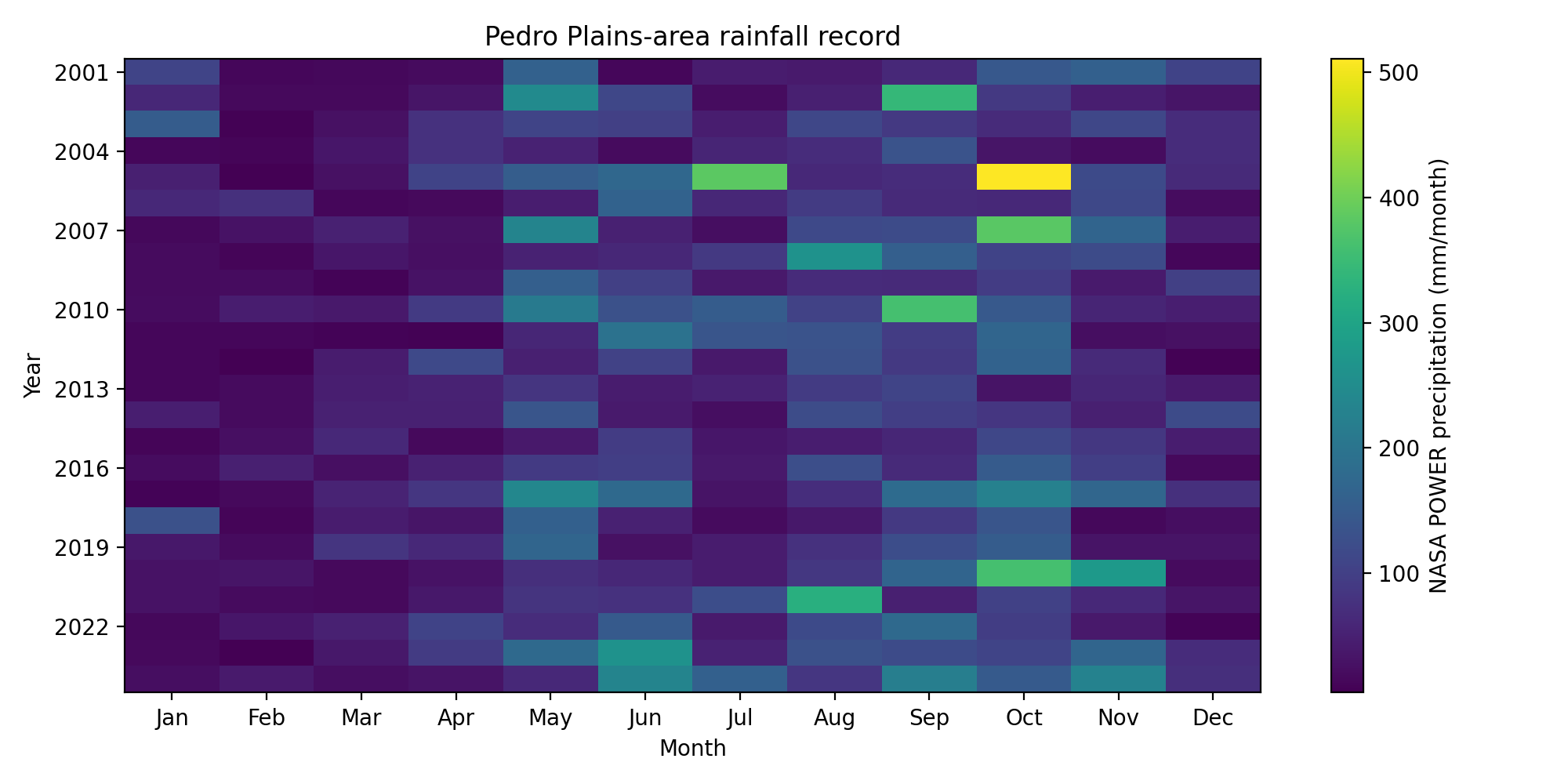
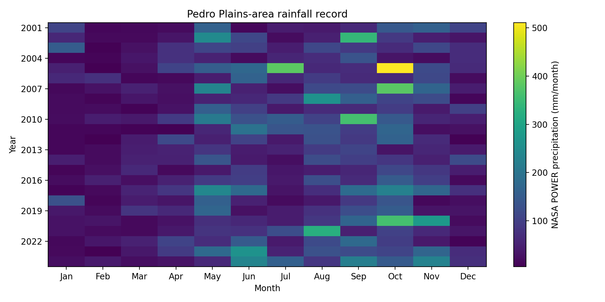
The sampling coordinate is N, W in the Pedro Plains area. It is not a surveyed farm or a parcel boundary. NASA POWER’s precipitation product draws on an assimilation model and represents its source grid, which can differ from a field [1], [2]. The downloaded response identifies MERRA2, corrected precipitation in mm/day and local solar time. It contains one nonnegative value per day from 1 January 2001 to 31 December 2024, including leap days. Acquisition and source hashes are preserved with the code.
This is real data obtained from a public scientific service; it is not local field ground truth. The analysis does not use the provider’s grid-average elevation as a soil or slope measurement. No field irrigation, rooting depth, soil-water capacity, cultivar, harvest, sales or pest records were available. Temperature and satellite reflectance do not enter this model.
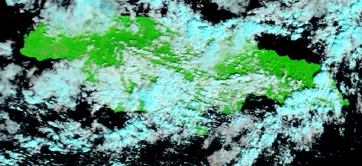
A companion animation replays the actual monthly rainfall values. A separate false-colour MODIS satellite image provides geographic context. It is not a rainfall map, crop-health estimate or validation layer. Keeping these roles separate prevents visual detail from suggesting evidence the model does not contain.
Information available at the decision
The training archive is fixed at 2001–2018. Each Monte Carlo draw selects a whole historical year with replacement and retains its daily rainfall sequence for the candidate planting window. This preserves within-season wet and dry runs better than independent daily resampling. It cannot create unseen extremes, and 5,000 draws do not create 5,000 distinct weather years: the weather support is eighteen years.
The same random draw of year, soil capacity, initial storage, demand and economic parameters is used across competing plans. Initial storage is reset to the same sampled fraction for every candidate; it is not reconstructed from the rainfall before each planting date. This isolates candidate sensitivity but omits antecedent-moisture differences. Pairing isolates changes attributable to the candidate choice within the assumed simulator. Selection maximises mean simulated margin using only training years. The chosen plan is then evaluated against the baseline under each of six held-out rainfall years, 2019–2024. It is not reselected after seeing those years.
This prevents future valid-time rainfall from choosing the plan. It does not reproduce the exact data product available in March of each historical year: the reanalysis was retrieved in 2026. The exercise is a retrospective information-cutoff test, not an archived real-time forecast trial. Future work must freeze acquisition vintages and operational forecast issue times.
Water balance and crop response
Let denote available soil water, rainfall and daily applied irrigation, all in mm. Soil capacity is and potential daily crop demand is . The daily calculation is Here combines unresolved overflow losses and is realised water use. No catchment routing, groundwater or infiltration-limited runoff is represented. The simulator maintains nonnegative storage and an explicit water balance.
The assumed relative yield response is The Food and Agriculture Organization’s seasonal response factors are for tomato and for watermelon [3]. These are general reference values, not local calibrations. Constant demand is a deliberate simplification; actual demand and sensitivity change with growth stage [4]. Severe deficits, excess water, disease and heat can invalidate this yield approximation. The computed is a simulated fraction of potential yield, not an observed harvest.
The prototype uses 90 days for tomato and 75 for watermelon, informed by the approximate maturity periods in official production material [5], [6]. The simulation ends at first maturity and does not model the later reaping period. The referenced budgets are historical; their monetary figures are not used as current quotes.
Monte Carlo assumptions and value
The code samples independent uniform ranges for capacity (60–140 mm), initial storage (25–75% of capacity), demand (3–5 mm/day), potential gross revenue (USD 3,000–9,000 per hectare), fixed cost (USD 1,500–4,500 per hectare) and delivered water cost (USD 0.10–0.60 per cubic metre). Each plan uses 0, 1 or 2 mm/day of irrigation. These ranges are illustrative inputs, not estimated local distributions. In particular, revenue and cost are assigned the same ranges to both crops to isolate model behaviour, not to compare their market profitability.
For a one-hectare plot, the scenario margin is The conversion factor is ten cubic metres per hectare per millimetre. The potential value of a choice is the paired difference . It is conditional on the assumed prices, water access and crop response. Neither a sales forecast nor a causal benefit is estimated. The reported 5th–95th percentiles describe scenario dispersion, not statistical confidence in a real farmer’s outcome.
Irrigation is treated as feasible and available every day; capital installation, credit, equipment failure and supply restrictions are absent. Crop price is held constant across dates and weather years. A market glut can make a water-secure crop unprofitable, as official reporting on St Elizabeth tomatoes illustrates [7]. A usable tool must therefore let the grower change the economics and refuse a recommendation when feasibility is unknown.
Executed framework results
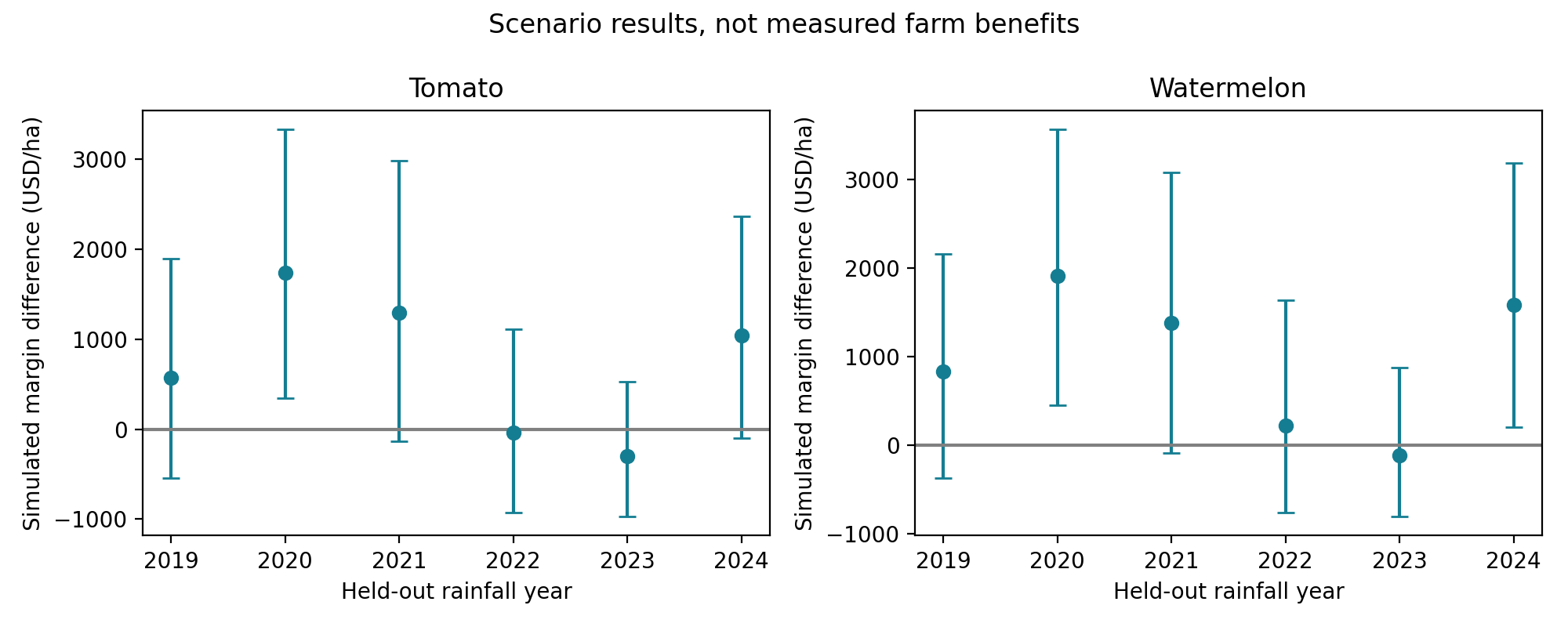
There are nine candidate plans per crop and 5,000 paired draws per candidate. Under the stated assumptions, both crops select 1 May with 2 mm/day irrigation. Relative to 1 April rainfed, mean training-scenario margin differences are USD 865/ha for tomato and USD 1,097/ha for watermelon. Their 5th–95th percentile differences span approximately USD -671 to USD 2,760 and USD -537 to USD 3,190 respectively. Negative cases remain material.
Across the six held-out rainfall years, mean simulated differences are USD 718/ha and USD 970/ha. These values describe a model experiment with real rainfall forcing and assumed crop economics. They are not evidence that a farmer earned or would earn those amounts. Figure 2 shows year-specific dispersion rather than hiding it behind the average.
Every simulated day passed storage bounds and water-accounting checks. Date uniqueness, nonnegative rainfall, training cutoff and identical-plan paired differences were also checked. These establish arithmetic and information separation within the code; they do not validate the crop model. The full candidate and held-out results are supplied as tables so adverse results remain visible.
Post hoc sensitivity to water cost and feasibility
A separate 60-setting stress grid varies the assumed potential-revenue scale (0.5, 1 or 1.5), deterministic water cost (USD 0, 0.35, 0.70, 1.40 or 2.80 per cubic metre) and eligibility of irrigation. Its design followed the original results, so it is exploratory rather than a fresh holdout. It reuses only training weather. Repeated rainfed results across water-price settings are not independent experiments.
At the original revenue scale, increasing water cost from USD 0.35 to 0.70 per cubic metre changes the highest-mean candidate to 15 April with 1 mm/day for tomato and 1 May with 1 mm/day for watermelon. At USD 1.40, both favour 15 April rainfed. With irrigation excluded, both also choose 15 April rainfed. Unknown water access therefore changes the candidate set, not merely a disclaimer below a recommendation.
The fixed 1 May/2 mm plan breaks even against 1 April rainfed at mean water prices of approximately USD 0.833 and 1.084 per cubic metre for tomato and watermelon. These are pairwise thresholds under the stated revenue assumptions, not globally optimal switching prices or local quotes. Shared fixed costs cancel. Extra capital expenditure would reduce these thresholds. Because the baseline remains eligible, the maximised mean difference cannot be negative; the archive separately reports draw-level downside and the original fixed plan’s losses.
A physics-informed neural surrogate experiment
A separate experiment asks whether a soft physical penalty improves a neural approximation of one bucket step. The five inputs are initial storage, daily precipitation, irrigation, capacity and demand. The three outputs are next-day storage, realised water use and overflow. All quantities are divided by 100 mm before training. The targets are computed by the equations above, not measured soil states or yields. This is a discrete-time, physics-informed neural surrogate; it does not solve a spatial partial differential equation.
Training inputs use rainfall dates from 2001–2015, with one independently sampled soil and management state per date. The 2016–2018 dates are excluded from fitting and no model selection uses them. Testing uses 2,192 daily rainfall inputs from 2019–2024 with separately sampled states. Both models receive the same 1,000 labelled training transitions, initial weights and minibatches within each seed. There is one 32-unit hyperbolic-tangent hidden layer and a linear output layer, giving 291 parameters. Three seeds (101, 202 and 303) each run 1,500 Adam steps at learning rate 0.003 and batch size 128. No hyperparameter search was conducted. The penalty adds unlabelled training-input information and extra gradient computation; the comparison matches supervised data and update count, not total computation or total constraint information.
With hats denoting predicted normalised outputs, the physical residual is The physics-informed loss adds the mean squared residual and squared violations of nonnegative outputs, storage capacity and demand bounds to the supervised mean squared error, each with unit weight. The data-only network has the same architecture and supervised loss without these penalties. An independent minibatch of training inputs supplies the residual evaluations. This is a soft constraint: no post-processing projection conceals violations.
Finite-difference checks of sampled gradient components gave maximum absolute discrepancy . Table 1 gives every seed rather than selecting the favourable run. The penalty reduces mass-balance root mean squared error in all three runs but worsens storage and realised-water-use errors in all three. Maximum absolute balance error also worsens in two seeds (202 and 303), despite the lower average squared residual. Negative outputs persist in 21.8–37.8% of test transitions for the penalised network, using a normalised numerical tolerance (equivalent to mm). Thus a lower conservation residual does not establish a physically admissible or more accurate surrogate.
| Seed | Model | Storage error (mm) | Balance error (mm) |
|---|---|---|---|
| 101 | Data only | 2.294 | 0.930 |
| 101 | Physics informed | 2.448 | 0.560 |
| 202 | Data only | 1.790 | 0.977 |
| 202 | Physics informed | 2.429 | 0.931 |
| 303 | Data only | 2.398 | 0.971 |
| 303 | Physics informed | 2.679 | 0.773 |
The exact bucket is already inexpensive and remains the scenario engine. This neural test establishes neither a speed advantage nor a reason to replace it. Autonomous rollouts, yield propagation and forecast performance were not tested. The comparison is exploratory: the wider programme had already inspected these historical years before this separate protocol was fixed, although test labels did not enter training or parameter selection.
Future work and field validation
A prospective extension requires soil-water measurements, planting dates, irrigation logs, cultivar details, harvested mass and realised prices from farms and extension partners. Rain-gauge comparisons would test the bias of the gridded rainfall input. No participant access, partnership or approval is claimed here.
A prospective study should freeze the data issue date, weather forecast, feasible candidate set and baseline before planting. It should compare the current bucket model with a calibrated crop model, historical-calendar advice and any proposed learned model under the same information. Calibration and test farms or seasons must remain separate. Primary outcomes should include yield error, water use, realised margin and decision regret; failed recommendations and adverse outcomes should be retained.
The next neural comparison should test exact architectural constraints, matched tuning budgets and multi-step stability before any decision engine is replaced. A separate interface study must measure whether users understand adverse cases and missing feasibility information. Agricultural tool uptake depends on relevance and usability as well as model performance [17]; better explanations do not automatically reduce overreliance [18]. Design guidance supports communicating limits and corrections [19], while risk-management guidance treats validation and contextual harms as separate responsibilities [20].
Conclusion and reproducibility
Actual rainfall forcing makes the scenario exercise reproducible but does not supply missing field outcomes. Water cost and feasibility alter the preferred plan, and a physics penalty improves the surrogate’s balance metric while worsening its storage accuracy. These results support retaining explicit baselines, adverse scenarios and separate physical checks before using a model in crop decisions.
The supporting material preserves the NASA response, acquisition URL, seeds, protocols, simulator, neural weights, all candidate results, sensitivity grid and checks. No personal farm records or human participants were used. No prospective field access or partnership is implied. The accompanying interface protocol shares this numerical experiment and is not an independent agronomic replication.
References
NASA POWER. Daily API documentation. Accessed 13 November 2026. https://power.larc.nasa.gov/docs/services/api/temporal/daily/.
NASA POWER. Data questions. Accessed 13 November 2026. https://power.larc.nasa.gov/docs/faqs/data/.
Food and Agriculture Organization. Annex II: Irrigation scheduling, Table 12 and Section 2.1. https://www.fao.org/4/X5647E/x5647e0e.htm.
Food and Agriculture Organization. Chapter 3: Crop water needs. https://www.fao.org/4/S2022E/s2022e07.htm.
Jamaica Ministry of Agriculture. Cost of production, 2023, tomato production information for St Elizabeth. https://www.moa.gov.jm/sites/default/files/pdfs/COP_2023.pdf.
Jamaica Ministry of Agriculture. Cost of production, 2017, watermelon production information for Pedro Plain. https://moa.gov.jm/sites/default/files/pdfs/COP_2017_combined.pdf.
Jamaica Ministry of Agriculture, Fisheries and Mining. RADA moves to address tomato glut amid surge in production. 7 March 2025. https://www.moa.gov.jm/content/rada-moves-address-tomato-glut-amid-surge-production.
Food and Agriculture Organization. About AquaCrop: crop water productivity model. https://www.fao.org/aquacrop/overview/en/. Accessed 13 November 2026.
J. W. Jones et al. (2003). The DSSAT cropping system model. European Journal of Agronomy 18, 235–265. https://doi.org/10.1016/S1161-0301(02)00107-7.
R. G. Allen, L. S. Pereira, D. Raes and M. Smith (1998). Crop evapotranspiration: guidelines for computing crop water requirements. FAO Irrigation and Drainage Paper 56. https://www.fao.org/4/X0490E/x0490e00.htm.
P. Steduto, T. C. Hsiao, E. Fereres and D. Raes (2012). Crop yield response to water. FAO Irrigation and Drainage Paper 66. https://www.fao.org/4/i2800e/i2800e00.htm.
D. Rankine et al. (2021). Evaluation of DSSAT-MANIHOT-Cassava model to determine potential irrigation benefits for cassava in Jamaica. Agronomy Journal 113, 5317–5334. https://doi.org/10.1002/agj2.20876.
M. Raissi, P. Perdikaris and G. E. Karniadakis (2019). Physics-informed neural networks: a deep learning framework for solving forward and inverse problems involving nonlinear partial differential equations. Journal of Computational Physics 378, 686–707. https://doi.org/10.1016/j.jcp.2018.10.045.
T. Beucler et al. (2021). Enforcing analytic constraints in neural networks emulating physical systems. Physical Review Letters 126, 098302. https://doi.org/10.1103/PhysRevLett.126.098302.
A. Krishnapriyan, A. Gholami, S. Zhe, R. Kirby and M. W. Mahoney (2021). Characterizing possible failure modes in physics-informed neural networks. Advances in Neural Information Processing Systems 34. https://papers.nips.cc/paper/2021/hash/df438e5206f31600e6ae4af72f2725f1-Abstract.html.
A. Dunkley (2026). Exact volume conservation improves a neural rainfall downscaler over Jamaica and does not beat seasonal allocation: a conditional CHIRPS benchmark with a driver-error floor. Unpublished research manuscript, 10 November.
D. C. Rose et al. (2016). Decision support tools for agriculture: towards effective design and delivery. Agricultural Systems 149, 165–174. https://doi.org/10.1016/j.agsy.2016.09.009.
Z. Buçinca, M. B. Malaya and K. Z. Gajos (2021). To trust or to think: cognitive forcing functions can reduce overreliance on AI in AI-assisted decision-making. Proceedings of the ACM on Human-Computer Interaction 5(CSCW1). https://doi.org/10.1145/3449287.
S. Amershi et al. (2019). Guidelines for human-AI interaction. CHI. https://doi.org/10.1145/3290605.3300233.
National Institute of Standards and Technology (2023). Artificial Intelligence Risk Management Framework. NIST AI 100-1. https://doi.org/10.6028/NIST.AI.100-1.